The other day I had estimates from several logistic regression models, and I wanted to superimpose the univariate KDE’s of the predictions. The outcome was fairly rare, so the predictions were bunched up at the lower end of the probability scale, and the default kernel density estimates on the probability scale smeared too much of the probability outside of the range.

It is a general problem with KDE estimates, and there are two general ways to solve it:

• truncate the KDE and then reweight the points near the edge (example)
• estimate the KDE on some other scale that does not have a restricted domain, and then transform the density back to the domain of interest (example)

The first is basically the same as edge correction in spatial statistics, just in one dimension instead of the two. Here I will show how to do the second in R, mapping items on the logistic scale to the probability scale. The second linked CV post shows how to do this when using the log transformation, and here I will show the same with mapping logistic estimates (e.g. from the output of a logistic regression model). This requires the data to not have any values at 0 or 1 on the probability scale, because these will map to negative and positive infinity on the logistic scale.

In R, first define the logit function as log(p/(1-p) and the logistic function as 1/(1+exp(-x)) for use later:

logistic <- function(x){1/(1+exp(-x))}
logit <- function(x){log(x/(1-x))}

We can generate some fake data that might look like output from a logistic regression model and calculate the density object.

set.seed(10)
x <- rnorm(100,0,0.5)
l <- density(x)  #calculate density on logit scale

This blog post goes through the necessary math, but in a nut shell you can’t simply just transform the density estimate using the same function, you need to apply an additional transformation (referred to as the Jacobian). So here is an example transforming the density estimate from the logistic scale, l above, to the probability scale.

px <- logistic(l$x)  #transform density to probability scale
py <- l$y/(px*(1-px))
plot(px,py,type='l')

To make sure that the area does sum to one, we can superimpose the density calculated on the data transformed to the probability scale. In this example of fake data the two are pretty much identical. (Black line is my transformed density, and the red is the density estimate based on the probability data.)

dp <- density(logistic(x)) #density on the probability values to begin with
lines(dp$x,dp$y,col='red')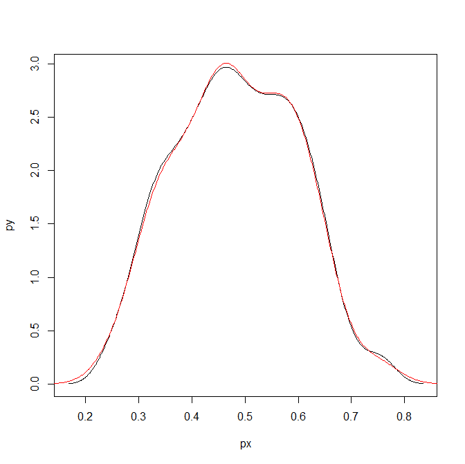

Here is a helper function, denLogistic, to do this in the future, which simply takes the data (on the logistic scale) and returns a density object modified to the probability scale.

logistic <- function(x){1/(1+exp(-x))}
logit <- function(x){log(x/(1-x))}
denLogistic <- function(x){
  d <- density(x)
  d$x <- logistic(d$x)
  d$y <- d$y/(d$x*(1-d$x))
  d$call <- 'Logistic Density Transformed to Probability Scale'
  d$bw <- paste0(signif(d$bw,4)," (on Logistic scale)")
  return(d)
}

In cases where more of the probability density is smeared beyond 0-1 on the probability scale, the logistic density estimate will look different. Here is an example with a wider variance and more predictions near zero, so the two estimates differ by a larger amount.

lP <- rnorm(100,-0.9,1)
test <- denLogistic(lP)
plot(test)
lines(density(logistic(lP)),col='red')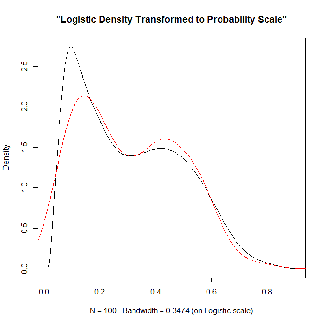

Again, this works well for data on the probability scale that can not be exactly zero or one. If you have data like that, the edge correction type KDE estimators are better suited.