Weighted buffers in R

Had a request not so recently about implementing weighted buffer counts. The idea behind a weighted buffer is that instead of say counting the number of crimes that happen within 1,000 meters of a school, you want to give events that are closer to the school more weight.

There are two reasons you might want to do this for crime analysis:

  • You want to measure the amount of crime around a location, but you rather have a weighted crime count, where crimes closer to the location have a greater weight than those further away.
  • You want to measure attributes nearby a location (so things that predict crime), but give a higher weight to those closer to a location.

The second is actually more common in academic literature — see John Hipp’s Egohoods, or Liz Groff’s work on measuring nearby to bars, or Joel Caplan and using kernel density to estimate the effect of crime generators. Jerry Ratcliffe and colleagues work on the buffer intensity calculator is actually the motivation for the original request. So here are some quick code snippets in R to accomplish either. Here is the complete code and original data to replicate.

Here I use over 250,000 reported Part 1 crimes in DC from 08 through 2015, 173 school locations, and 21,506 street units (street segment midpoints and intersections) I constructed for various analyses in DC (all from open data sources) as examples.

Example 1: Crime Buffer Intensities Around Schools

First, lets define where our data is located and read in the CSV files (don’t judge me setting the directory, I do not use RStudio!)

MyDir <- 'C:\\Users\\axw161530\\Dropbox\\Documents\\BLOG\\buffer_stuff_R\\Code' #Change to location on your machine!
setwd(MyDir)

CrimeData <- read.csv('DC_Crime_08_15.csv')
SchoolLoc <- read.csv('DC_Schools.csv')

Now there are several ways to do this, but here is the way I think will be most useful in general for folks in the crime analysis realm. Basically the workflow is this:

  • For a given school, calculate the distance between all of the crime points and that school
  • Apply whatever function to that distance to get your weight
  • Sum up your weights

For the function to the distance there are a bunch of choices (see Jerry’s buffer intensity I linked to previously for some example discussion). I’ve written previously about using the bi-square kernel. So I will illustrate with that.

Here is an example for the first school record in the dataset.

#Example for crimes around school, weighted by Bisquare kernel
BiSq_Fun <- function(dist,b){
    ifelse(dist < b, ( 1 - (dist/b)^2 )^2, 0)
    }

S1 <- t(SchoolLoc[1,2:3])
Dis <- sqrt( (CrimeData$BLOCKXCOORD - S1[1])^2 + (CrimeData$BLOCKYCOORD - S1[2])^2 )
Wgh <- sum( BiSq_Fun(Dis,b=2000) )

Then repeat that for all of the locations that you want the buffer intensities, and stuff it in the original SchoolLoc data frame. (Takes less than 30 seconds on my machine.)

SchoolLoc$BufWeight <- -1 #Initialize field

#Takes about 30 seconds on my machine
for (i in 1:nrow(SchoolLoc)){
  S <- t(SchoolLoc[i,2:3])
  Dis <- sqrt( (CrimeData$BLOCKXCOORD - S[1])^2 + (CrimeData$BLOCKYCOORD - S[2])^2 )
  SchoolLoc[i,'BufWeight'] <- sum( BiSq_Fun(Dis,b=2000) )
}

In this example there are 173 schools and 276,621 crimes. It is too big to create all of the pairwise comparisons at once (which will generate nearly 50 million records), but the looping isn’t too cumbersome and slow to worry about building a KDTree.

One thing to note about this technique is that if the buffers are large (or you have locations nearby one another), one crime can contribute to weighted crimes for multiple places.

Example 2: Weighted School Counts for Street Units

To extend this idea to estimating attributes at places just essentially swaps out the crime locations with whatever you want to calculate, ala Liz Groff and her inverse distance weighted bars paper. I will show something alittle different though, in using the weights to create a weighted sum, which is related to John Hipp and Adam Boessen’s idea about Egohoods.

So here for every street unit I’ve created in DC, I want an estimate of the number of students nearby. I not only want to count the number of kids in attendance in schools nearby, but I also want to weight schools that are closer to the street unit by a higher amount.

So here I read in the street unit data. Also I do not have school attendance counts in this dataset, so I just simulate some numbers to illustrate.

StreetUnits <- read.csv('DC_StreetUnits.csv')
StreetUnits$SchoolWeight <- -1 #Initialize school weight field

#Adding in random school attendance
SchoolLoc$StudentNum <- round(runif(nrow(SchoolLoc),100,2000)) 

Now it is very similar to the previous example, you just do a weighted sum of the attribute, instead of just counting up the weights. Here for illustration purposes I use a different weighting function, inverse distance weighting with a distance cut-off. (I figured this would need a better data management strategy to be timely, but this loop works quite fast as well, again under a minute on my machine.)

#Will use inverse distance weighting with cut-off instead of bi-square
Inv_CutOff <- function(dist,cut){
    ifelse(dist < cut, 1/dist, 0)
}

for (i in 1:nrow(StreetUnits)){
    SU <- t(StreetUnits[i,2:3])
    Dis <- sqrt( (SchoolLoc$XMeters - SU[1])^2 + (SchoolLoc$YMeters - SU[2])^2 )
    Weights <- Inv_CutOff(Dis,cut=8000)
    StreetUnits[i,'SchoolWeight'] <- sum( Weights*SchoolLoc$StudentNum )
}   

The same idea could be used for other attributes, like sales volume for restaurants to get a measure of the business of the location (I think more recent work of John Hipp’s uses the number of employees).

Some attributes you may want to do the weighted mean instead of a weighted sum. For example, if you were using estimates of the proportion of residents in poverty, it makes more sense for this measure to be a spatially smoothed mean estimate than a sum. In this case it works exactly the same but you would replace sum( Weights*SchoolLoc$StudentNum ) with sum( Weights*SchoolLoc$StudentNum )/sum(Weights). (You could use the centroid of census block groups in place of the polygon data.)

Some Wrap-Up

Using these buffer weights really just swaps out one arbitrary decision for data analysis (the buffer distance) with another (the distance weighting function). Although the weighting function is more complicated, I think it is probably closer to reality for quite a few applications.

Many of these different types of spatial estimates are all related to another (kernel density estimation, geographically weighted regression, kriging). So there are many different ways that you could go about making similar estimates. Not letting the perfect be the enemy of the good, I think what I show here will work quite well for many crime analysis applications.

Turning SPSS data into Python data

Previously I blogged about how to take Python data and turn it back into SPSS data. Here we are going to do the opposite — turn SPSS data into Python objects. First to start out we will make a simple dataset of three variables.

DATA LIST Free /X Y (2F1.0) Z (A1). 
BEGIN DATA
1 2 A
4 5 B
7 8 C
END DATA.
DATASET NAME Test.
EXECUTE.

To import this data into Python, we need to import the spss class of functions, which then you can read cases from the active dataset using the Cursor attribute. Here is an example of grabbing all of the cases.

*Importing all of the data.
BEGIN PROGRAM Python.
import spss
dataCursor = spss.Cursor()
AllData = dataCursor.fetchall()
dataCursor.close()
print AllData
END PROGRAM.

What this then prints out is ((1.0, 2.0, 'A'), (4.0, 5.0, 'B'), (7.0, 8.0, 'C')), a set of nested tuples. You can also just grab one case by replacing dataCursor.fetchall() with dataCursor.fetchone(), in which case it will just return one tuple.

To only grab particular variables from the list, you can pass a set of indices in the spss.Cursor object. Remember, Python indices start at zero, so if you want the first and second variables in the dataset, you need to grab the 0 and 1 indices.

*Only grabbing certain variables.
BEGIN PROGRAM Python.
dataNum = spss.Cursor([0,1])
spNumbers = dataNum.fetchall()
dataNum.close()
print spNumbers
END PROGRAM.

This subsequently prints out ((1.0, 2.0), (4.0, 5.0), (7.0, 8.0)). When grabbing one variable, you may want just a list of the objects instead of the nested tuples. Here I use list comprehension to turn the resulting tuples for the Z variable into a nice list.

*Converting to a nice list.
BEGIN PROGRAM Python.
dataAlp = spss.Cursor([2])
spAlp = dataAlp.fetchall()
dataAlp.close()
spAlp_list = [i[0] for i in spAlp] #convert to nice list
print spAlp
print spAlp_list
END PROGRAM.

The first print object is (('A',), ('B',), ('C',)), but the second is ['A', 'B', 'C'].

The above code works fine if you know the position of the variable in the file, but if the position can change this won’t work. Here is a one liner to get the variable names of the active dataset and plop them in a list.

*Way to get SPSS variable names.
BEGIN PROGRAM Python.
varList = [spss.GetVariableName(i) for i in range(spss.GetVariableCount())]
print varList
END PROGRAM.

Now if you have your list of variable names you want, you can figure out the index value. There are two ways to do it, iterate over the list of variable names in the dataset, or iterate over the list of your specified variables. I do the latter here (note this will result in an error if you supply a variable name not in the dataset).

*Find the indices of specific variables.
BEGIN PROGRAM Python.
LookVars = ["X","Z"]
VarInd = [varList.index(i) for i in LookVars]
print VarInd
END PROGRAM.

Now you can just supply VarInd above to the argument for spss.Cursor to grab those variables. Here I wrapped it all up in a function.

*Easy function to use.
BEGIN PROGRAM Python.
import spss
def AllSPSSdat(vars):
  if vars == None:
    varNums = range(spss.GetVariableCount())
  else:
    allvars = [spss.GetVariableName(i) for i in range(spss.GetVariableCount())]
    varNums = [allvars.index(i) for i in vars]
  data = spss.Cursor(varNums)
  pydata = data.fetchall()
  data.close()
  return pydata
END PROGRAM.

You can either supply a list of variables or None, in the latter case all of the variables are returned.

BEGIN PROGRAM Python.
MyDat = AllSPSSdat(vars=["Y","Z"])
print MyDat
END PROGRAM.

This set of nested tuples is then pretty easy to convert to other Python objects. Panda’s dataframes, Numpy arrays, and NetworkX objects are all one liners. Here is turning the entire dataset into a panda’s data frame.

*Turn into pandas data frame.
BEGIN PROGRAM Python.
import pandas as pd
MyDat = AllSPSSdat(vars=None)
allvars = [spss.GetVariableName(i) for i in range(spss.GetVariableCount())]
PanDat = pd.DataFrame(list(MyDat),columns=allvars)
print PanDat
END PROGRAM.

Which prints out.

   X  Y  Z 
0  1  2  A 
1  4  5  B 
2  7  8  C

Using KDTree’s in python to calculate neighbor counts

For a few different projects I’ve had to take a set of crime data and calculate the number of events nearby. It is a regular geospatial task, counting events in a particular buffer, but one that can be quite cumbersome if you have quite a few points to cross-reference. For one project I needed to calculate this for 4,500 street segments and intersections against a set of over 100,000 crime incidents. While this is not big data, if you go the brute force route and simply calculate all pair-wise distances, this results in 450 million comparisons. Since all I wanted was the number of counts within a particular distance buffer, KDTree’s offer a much more efficient search solution.

Here I give an example in Python using numpy and the nearest neighbor algorithms available in SciPy. This example is calculating the number of shootings in DC within 1 kilometer of schools. The shooting data is sensor data via ShotSpotter, and is publicly available at the new open data site. The school data I calculated the centroids based on school area polygons, available from the legacy DC data site. This particular example was motivated by this Urban Institute post.

There are around 170 schools and under 40,000 total shootings, so this would not be a big issue to calculate all the pairwise distances. It is a simple and quick example though. Here I have the Python code and CSV files are available to download.

So first we will just import the spatial data into numpy arrays. Note each file has the coordinates in projected meters.

import numpy as np
#getting schools and shootings from CSV files
schools = np.genfromtxt('DC_Schools.csv', delimiter=",", skip_header=1)
shootings = np.genfromtxt('ShotSpotter.csv', delimiter=",", skip_header=1, usecols=(4,5))

Next we can import the KDTree function, and then supply it with the two spatial coordinates for the shootings. While this is a relatively small file, even for my example larger set of crime data with over 100,000 incidents building the tree was really fast, less than a minute.

#making KDTree, and then searching within 1 kilometer of school
from sklearn.neighbors import KDTree
shoot_tree = KDTree(shootings)

Finally you can then search within a particular radius. You can either search one location at a time, but here I do a batch search and count the number of shootings that are within 1,000 meters from each school. Again this is a small example, but even with my 4,500 locations against 100,000 crimes it was very fast. (Whereas my initial SPSS code to do all 450 million pairwise combinations was taking all night.)

shoot_tree.query_radius(schools[:,[1,2]],r=1000,count_only=True)

Which produces an array of the counts for each of the schools:

array([1168,  179, 2384,  686,  583, 1475,  239, 1890, 2070,  990,   74,
        492,   10,  226, 2057, 1813, 1137,  785,  742, 1893, 4650, 1910,
          0,  926, 2380,  818, 2868, 1230,    0, 3230, 1103, 2253, 4531,
       1548,    0,    0,    0, 1002, 1912,    0, 1543,    0,  580,    4,
       1224,  843,  212,  591,    0,    0, 1127, 4520, 2283, 1413, 3255,
        926,  972,  435, 2734,    0, 2828,  724,  796,    1, 2016, 2540,
        369, 1903, 2216, 1697,  155, 2337,  496,  258,  900, 2278, 3123,
        794, 2312,  636, 1663,    0, 4896,  604, 1141,    7,    0, 1803,
          2,  283,  270, 1395, 2087, 3414,  143,  238,  517,  238, 2017,
       2857, 1100, 2575,  179,  876, 2175,  450, 5230, 2441,   10, 2547,
        202, 2659, 4006, 2514,  923,    6, 1481,    0, 2415, 2058, 2309,
          3, 1132,    0, 1363, 4701,  158,  410, 2884,  979, 2053, 1120,
       2048, 2750,  632, 1492, 1670,  242,  131,  863, 1246, 1361,  843,
       3567, 1311,  107, 1501,    0, 2176,  296,  803,    0, 1301,  719,
         97, 2312,  150,  475,  764, 2078,  912, 2943, 1453,  178,  177,
        389,  244,  874,  576,  699,  295,  843,  274])

And that is it! Quite simple.

The ShotSpotter data is interesting, with quite a few oddities that are worth exploring. I recently wrote a chapter on SPSS’s geospatial tools for an upcoming book on advanced SPSS features, providing a predictive police example predicting weekly shootings using the new geospatial temporal modelling tool. The book is edited by Keith McCormick and Jesus Salcedo, and I will write a blog post whenever it comes out highlighting what the chapter goes over.

Using local Python objects in SPSSINC TRANS – examples with network statistics

When using SPSSINC TRANS, you have a wider array of functions to compute on cases in SPSS. Within the local session, you can create your own python functions within a BEGIN PROGRAM and END PROGRAM block. In SPSSINC TRANS you pass in the values in the current dataset, but you can also create functions that use data in the local python environment as well. An example use case follows in which you create a network in the local python environment using SPSS data, and then calculate several network statistics on the nodes. Here is a simple hierarchical network dataset that signifies managers and subordinates in an agency.

*Edge list. 
DATA LIST FREE / Man Sub (2F1.0). 
BEGIN DATA 
1 2 
2 3 
2 4 
3 5 
3 6 
4 7 
4 8 
END DATA. 
DATASET NAME Boss. 

We can subsequently turn this into a NetworkX graph with the code below. Some of my prior SPSS examples using NetworkX had a bit more complicated code using loops and turning the SPSS dataset into the network object. But actually the way SPSS dumps the data in python (as a tuples nested within a list) is how the add_edges_from function expects it in NetworkX, so no looping required (and it automatically creates the nodes list from the edge data).

BEGIN PROGRAM Python. 
import networkx as nx
import spss, spssdata

alldata = spssdata.Spssdata().fetchall()  #get SPSS data
G = nx.DiGraph()                          #create empty graph
G.add_edges_from(alldata)                 #add edges into graph
print G.nodes()
END PROGRAM.

Note now that we have the graph object G in the local python environment for this particular SPSS session. We can then make our own functions that references G, but takes other inputs. Here I have examples for the geodesic distance between two nodes, closeness and degree centrality, and the average degree of the neighbors.

BEGIN PROGRAM Python.
#path distance
def geo_dist(source,target): 
  return nx.shortest_path_length(G,source,target)
#closeness centrality
def close_cent(v):
  return nx.closeness_centrality(G,v)
#degree
def deg(v):
  return G.degree(v)
#average degree of neighbors
def avg_neideg(v):
  return nx.average_neighbor_degree(G,nodes=[v])[v]
END PROGRAM.

Here is the node list in a second SPSS dataset that we will calculate the mentioned statistics on. For large graphs, this is nice because you can select out a smaller subset of nodes and only worry about the calculations on that subset. For a crime analysis example, I may be monitoring a particular set of chronic offenders, and I want to calculate how close every arrested person within the month is to the set of chronic offenders.

DATA LIST FREE / Employ (F1.0). 
BEGIN DATA 
1 
2
3
4
5
6
7
8
END DATA. 
DATASET NAME Emp. 
DATASET ACTIVATE Emp.

Now we have all the necessary ingredients to calculate our network statistics on these nodes. Here are examples of using SPSSINC TRANS to calculate the network statistics in the local SPSS dataset.

*Geodesic distance from 1.
SPSSINC TRANS RESULT=Dist TYPE=0
  /FORMULA "geo_dist(source=1.0,target=Employ)".

*closeness centrality.
SPSSINC TRANS RESULT=Cent TYPE=0
  /FORMULA "close_cent(v=Employ)".

*degree.
SPSSINC TRANS RESULT=Deg TYPE=0
  /FORMULA "deg(v=Employ)".

*Average neighbor degree.
SPSSINC TRANS RESULT=NeighDeg TYPE=0
  /FORMULA "avg_neideg(v=Employ)".

Some ad-hoc fuzzy name matching within Police databases

A repeated annoying task I have had to undertake is take a list of names and date-of-births and match them to a reference set. This can happen when you try to merge data from different sources. Or when working with police RMS data, a frequent problem is the same individual can go into the master name list multiple times. This can be either due to data error, or someone being malicious and providing the PD with fraudulent data.

Most often I am trying to match a smaller set of names to a bigger set from a police RMS system. Typically what I do is grab all of the names in the police RMS, make them the same case, and then simply sort the file by last then first name. Then I typically go through one by one from the smaller file and identify the name ID’s that are in the sorted bigger police database. Ctrl-F can make it a quick search for only a few people.

This works quite well for small numbers, but I wanted to see if I could make some simple rules when I need to match a larger list. For example, the above workflow may be fine if I need to look up 10 names quickly, but say you want to eliminate duplicates in the entire PD RMS system? A manually hand search through 100,000+ names is crazy (and will be out of date before you finish).

A tool I’ve used in the past (and would recommend) is FRIL, Fine-grained records integration and linkage tool. In a nutshell the way that tool works is that you can calculate string distances between names and/or date distances between date-of-births from two separate files. Then you specify how close you want the records to be to either automatically match the records or manually view and make a personal determination if the two records are the same person. FRIL has a really great interface to quickly view the suggested matches and manually confirm or reject certain matches.

FRIL uses the Potter Stewart I know it when I see it approach to finding matches. There is no ground truth, you just use your best judgement whether two names belong to the same person, and FRIL uses some metrics to filter out the most unlikely candidates. I have a bit of a unique strategy though to identify typical string and date of birth differences in fuzzy name matches by using Police RMS data itself. Police RMS’s tend to have a variety of people who are linked up to the same master name index value, but for potentially several reasons they have various idiosyncrasies among different individual incidents. This allows me to calculate distances within persons, so a ground truth estimate, and then I can evaluate different distances compared to a control sample to see how well they the metrics discriminate matches.

There can be several reasons for slightly different data among an individuals incidents in a police RMS, but that they end up being linked to the same person. One is that frequently RMS systems incorporate tables from several different data sources, dispatchers have their own CAD system, the PD has a system to type in paper records, custodial arrests/finger printing may have another system, etc. Merging this data into one RMS may simply cause differences in how the data is stored or even how particular fields tend to be populated in the database. A second reason is that individuals can be ex-ante associated to a particular master name index, but can still have differences is various person fields for any particular incident.

One simple example is that for an arrest report the offender may have an old address in the system, so the officer types in the new address. The same thing can happen to slight name changes or DOB changes. The master name index should update with the most recent info, but you have a record trail of all the minor variations through each incident. Depending on the type of involvement in an incident has an impact on what information is collected and the quality of that information as well. For example, if I was interviewed as a witness to a crime, I may just go down in the report as Andy Wheeler with no date of birth info. If I was arrested, someone would take more time to put in my full name, Andrew Wheeler, and my date of birth. But if the original person inputting the data took the time, they would probably realize I was the same person and associate me with the same master ID.

So I can look at these within ID changes to see the typical distances. What I did was take a name database from a police department I work with, make all pair-wise comparisons between unique names and date of births, and then calculate several string distances between the names and the date differences between listed DOB’s. I then made a randomly matched sample for a comparison group. For the database I was working with this ended up being over 100,000 people with the same ID, but different names/DOB’s somewhere in different incidents, with an average of between 2~3 different names/dob’s per person (so a sample of nearly 200,000 same name comparisons, two names only results in one comparison, but three names results in 3 comparisons). My control sample took one of these names person and matched another random person in the database as a control group, so I have a control group sample of over 100,000 cases.

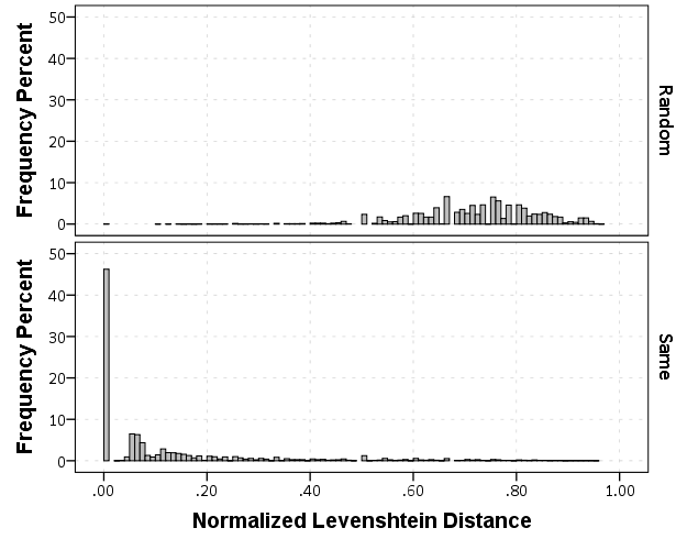
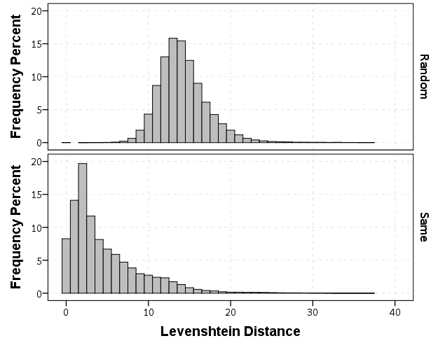
The data I was working with is secondary, so the names were already aggregated to Last, First Middle. If I had the original database I could do distances for the individual fields (and probably not worry about the middle name) but it somewhat simplifies the analysis as well. Here are some histograms of the Levenshtein distance between the name strings for the same person and random samples. The Levenshtein distance is the number of single edits it takes to transform one string to another string, so 0 would be the same word.

Part of the reason the distances within the same name have such a long tail is because of the already aggregated data. There end up being some people with full middle names, some with middle initials, and some with no middle names at all. So what I did was calculate a normalized Levenshtein distance based on the max and min possible values (listed at the Wikipedia page) the string can take given the size of the two input strings. The minimum value is the difference in the length of the two strings, the maximum is the length of the longest string. So then I calculate NormLevenDist = (LevenDist - min)/(max - min). This would cause Wheeler, Andy P and Wheeler, Andy Palmer to have a normalized distance of zero, whereas the edit distance would be 5. So in these histograms you can see even more discrimination between the two classes, based mainly on such names being perfect subsets of other names.

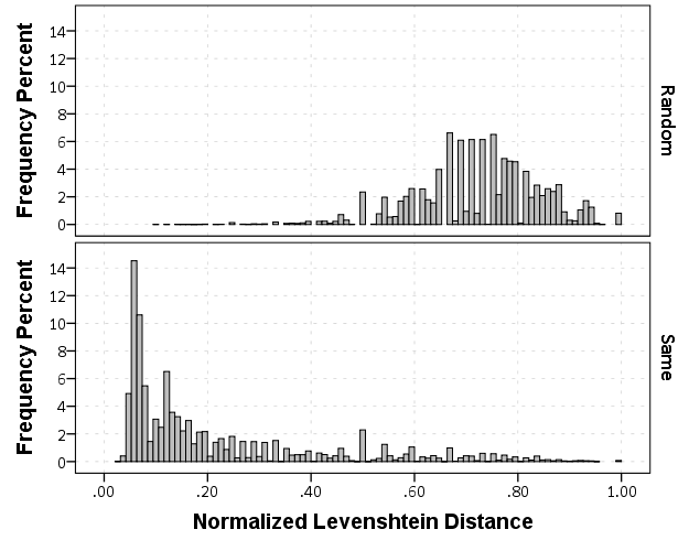
If you eliminate the 0’s in the normalized distance, you can get a better look at the shapes of each distribution. There is no clear cut-off between the samples, but there is a pretty clear difference in the distributions.

I also calculated the Jaro-Winkler and the Dice (bi-gram) string distances. All four of these metrics had a fairly high correlation, around 0.8 with one another, and all did pretty well classifying the same ID’s according to their ROC curves.

If I wanted to train a classifier as accurately as possible, I would use all of these metrics and probably make some sort of decision tree (or estimate their effects via logistic regression), but I wanted to make a simple function (since it will be doing quite a few comparisons) that calculates as few of the metrics as possible, so I just went with the normalized Levenshtein distance here. Jaro-Winkler would probably be more competitive if I had the separate first and last names (and played around with the weights for the beginning and ends of the strings). If you had mixed strings, like some are First Middle Last and others are Last First I suspect the dice similarity would be the best.

But in the end I think all of the string metrics will do a pretty similar job for this input data, and the normalized Levenshtein distance will work pretty well so I am going to stick with that. (I don’t consider soundex matching here, I’ve very rarely come across an example where soundex would match but had a high edit distance for names, e.g. typos are much more common than intentional mis-spellings based on enunciation I believe, and even the intentional mis-spellings tend to have a small edit distance.)

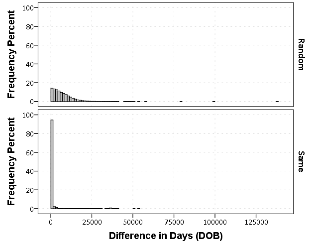
Now looking at the absolute differences in the DOB’s (where both are available) provides a bit of a different pattern. Here is the histograms

But I think the easiest illustration of this is to examine the frequency table of the most common day differences for the same individuals.

Obviously zero is the most common, but you can see a few other bumps that illustrate the nature of data mistakes. The second is 365 days – exactly off by one year. Also in the top 10 are 366, 731 & 730 – off by either a year and a day or two years. 1096, 1095, 1461, 1826, are examples of these yearly cycles as well. 36,525 are examples of being off by a century! Somewhere along the way some of the DOB fields were accidentally assigned to dates in the future (such as 2032 vs. 1932). The final examples are off by some other number typical of a simple typo, such as 10, 20, or by the difference in one month 30,31,27. By the end of this table of PDF of the same persons is smaller than the PDF of the control sample.

I also calculated string distances by transforming the DOB’s to mm/dd/yy format, but when incorporating the yearly cycles and other noted mistakes they did not appear to offer any new information.

So based on this information, I made a set of ad-hoc rules to classify matched names. I wanted to keep the false positive rate at less than 1 in 1,000, but make the true positive as high as possible. The simple rules I came up with were:

  • If a normalized Levenshtein distance of less than 0.2, consider a match
  • If a normalized Levenshtein distance of less than 0.4 and a close date, consider a match.

Close dates are defined as:

  • absolute difference of within 10 days OR
  • days apart are 10,20,27,30,31 OR
  • the number of days within a yearly cycle are less than 10

This match procedure produces the classification table below:

The false positive rate is right where I wanted it to be, but the true positive is a bit lower than I hoped. But it is a simple tool though to implement, and built into it you can have missing data for a birthday.

It is a bit hard to share this data and provide reproducible code, but if you want help doing something similar with your own data just shoot me an email and I will help. This was all done in SPSS and Python (using the extended transforms python code). In the end I wanted to make a simple Python function to use with the FUZZY command to automatically match names.

Passing arguments to SPSSINC TRANS (2)

Jon Peck made some great comments on my prior post on passing arguments to the SPSSINC TRANS function. Besides advice on that I should be quoting the argument on the FORMULA statement, he gave examples of how you can use the "TO" argument in both passing variables lists within the python formula and assigning variables to the results. Here is a brief example of their use.

First I will be working with a tiny, toy dataset:

DATA LIST FREE / X1 TO X4.
BEGIN DATA
1 2 3 4
5 6 7 8
9 8 7 6
5 4 3 2
END DATA.
DATASET NAME Test.

Now here is a command that returns the second lowest value in a list. (While there are plenty of things you can do in base code, this python code is very simple compared to what you would have to do in vanilla SPSS to figure this out.) In a nutshell you can specify the variable list on the /VARIABLE subcommand (and mix in TO to specify adjacent variables as in most SPSS commands). And then insert these into the python formula by specifying <>.

SPSSINC TRANS RESULT = Second
  /VARIABLES X1 TO X4
  /FORMULA "sorted([<>])[1]".

In my prior post, I showed how you could do this for the original variables, which would look like /FORMULA "sorted([X1,X2,X3,X4])[1]". Here you can see I’ve specified a set of variables on the VARIABLES subcommand, and inserted them into a list using [<>]. Enclosing <> in brackets produces a list in python. I then sort the list and grab the second element (located at 1, since python uses 0 based indices). You can also mix variables in the dataset and the <> listed on the variables subcommand. See here for an example.

You can also use the TO modifier in making a new set of variables. Here I return the sorted variables X1 TO X4 as a new set of variables S1 TO S4.

SPSSINC TRANS RESULT = S1 TO S4
  /VARIABLES X1 TO X4
  /FORMULA "sorted([<>])".

In both the prior examples I omitted the TYPE argument, as it defaults to 0 (i.e. a numeric variable returned as a float). But when specifying variable lists of the same type for multiple variables you can simply specify the type one time and the rest of the results are intelligently returned as the same. Here is the same sorted example, except that I return the results each as a string of length 1 as opposed to a numeric value.

SPSSINC TRANS RESULT = A1 TO A4 TYPE = 1
  /VARIABLES X1 TO X4 
  /FORMULA "map(str, sorted([<>]))".

Passing arguments to SPSSINC TRANS

So I actually bothered to read the help the other day for SPSSINC TRANS, which being generic allows you to use Python functions similar to how COMPUTE statements work, just a bit more general. Two examples of passing arguments I did not know you could do were 1) pass a list as an argument, and 2) pass constants that aren’t SPSS variables to functions. To follow are a few brief examples.

The first is passing a list to a function, and here is a simple example using the Python function sorted().

DATA LIST FREE / X1 X2 X3.
BEGIN DATA
3 2 1
1 0 3
1 1 2
2 2 1
3 0 3
END DATA.
DATASET NAME Test.

SPSSINC TRANS RESULT=S1 S2 S3 TYPE=0
  /FORMULA sorted([X1,X2,X3]).

This takes the variables X1 to X3, sorts them, and returns them in a new set of variables S1 to S3. We can also do reverse sorting by passing a constant value of 1 to the reverse function, which acts synonymously with reverse=True.

SPSSINC TRANS RESULT=RS1 RS2 RS3 TYPE=0
  /FORMULA sorted([X1,X2,X3],reverse=1).

This is a rather simplistic example, but the action is much simpler in Python than whatever equivalent SPSS code you can come up with. When using the SPSSINC TRANS extension it expects the returned function to simply be a flat list. For this sorting situation though it might be convenient to return the order in which the original value was stored. Here I make a function that returns the indice of the original list, and then flattens the two into sequential order, per this SO answer.

BEGIN PROGRAM Python.
import itertools

def SortList(L,reverse=0):
  I = range(1,len(L)+1)
  x = sorted(zip(L,I),reverse=reverse)
  r = list(itertools.chain.from_iterable(x))
  return r

#example use
print SortList(L=[2,1,3])
print SortList(L=[2,1,3],reverse=1)
END PROGRAM.

MATCH FILES FILE = * /DROP S1 TO RS3.

SPSSINC TRANS RESULT= S1 T1 S2 T2 S3 T3 TYPE=0
  /FORMULA SortList([X1,X2,X3],reverse=1).

When passing a string constant to a function in SPSSINC TRANS you need to triple quote the string. This makes some of my prior examples of using the Google maps related API’s much simpler. Instead of making variables to pass to the function, you can just triple quote the constants. Also when using the maps API I often have an argument for the API key, but you will get results even without a key (I presume Google just checks the IP address an limits you after so many requests). So for many of my functions you can not worry about making an API key and just pass an empty string. Here is an example from my prior Google distance API post using string constants and no API key.

BEGIN PROGRAM Python.
import urllib, json

#This parses the returned json to pull out the distance in meters and
#duration in seconds, [None,None] is returned is status is not OK
def ExtJsonDist(place):
  if place['rows'][0]['elements'][0]['status'] == 'OK':
    meters = place['rows'][0]['elements'][0]['distance']['value']
    seconds = place['rows'][0]['elements'][0]['duration']['value']
  else:
    meters,seconds = None,None
  return [meters,seconds]

#Takes a set of lon-lat coordinates for origin and destination,
#plus your API key and returns the json from the distance API
def GoogDist(OriginX,OriginY,DestinationX,DestinationY,key):
  MyUrl = ('https://maps.googleapis.com/maps/api/distancematrix/json'
           '?origins=%s,%s'
           '&destinations=%s,%s'
           '&key=%s') % (OriginY,OriginX,DestinationY,DestinationX,key)
  response = urllib.urlopen(MyUrl)
  jsonRaw = response.read()
  jsonData = json.loads(jsonRaw)
  data = ExtJsonDist(jsonData)
  return data
END PROGRAM.

*Grab the online data.
DATASET CLOSE ALL.
SPSSINC GETURI DATA
URI="https://dl.dropboxusercontent.com/u/3385251/NewYork_ZipCentroids.sav"
FILETYPE=SAV DATASET=NY_Zips.

*Selecting out only a few.
SELECT IF $casenum <= 5.
EXECUTE.

SPSSINC TRANS RESULT=Meters Seconds TYPE=0 0 
/FORMULA GoogDist(OriginX=LongCent,OriginY=LatCent,DestinationX='''-78.276205''',DestinationY='''42.850721''',key=''' ''').

Extracting items from SPSS tables using Python

Sometimes there are calculations provided for in SPSS tables that are necessary to use for other calculations. A frequent one is to grab certain percentiles from a FREQUENCY table (Equal Probability Histograms in SPSS is one example). The typical way to do this is to grab the table using OMS, but where that is overkill is if you need to merge this info. back into the original data for further calculations. I will show a brief example of grabbing the 25th, 50th, and 75th percentiles from a frequency table and using Python to calculate a robust standardized variable using these summary statistics.

First we will make a set of random data to work with.

SET SEED 10.
MATRIX.
SAVE {UNIFORM(100,1)} /OUTFILE = *.
END MATRIX.
DATASET NAME U.
FREQ COL1 /FORMAT = NOTABLE /PERCENTILES = 25 50 75.

The frequency table we are working with then looks like:

Now to get to the items in this frequency table we just to do a bit of going down a rabbit hole of different python objects.

  • The first block grabs the items in the output, which include tables and text.
  • The second block then grabs the last table for this specific output. Note that minus 2 from the size of the list is necessary because Python uses zero based indices and there is a log item after the table. So if the size of the list is 10, that means list[9] is the last item in the list. (Using negative indices does not work for extracting from the OutputItemList object.)
  • The third part then grabs the quantiles from the indices of the table. It ends up being in the first data column (so zero) and in the 3rd, 4th and 5th rows (again, Python uses zero based indices). Using GetUnformattedValueAt grabs the floating point number.
  • The final part then uses these quantiles to calculate a robust normalized variable by using spss.Submit and string substitution. (And then closes the SPSS client at the end.)

BEGIN PROGRAM Python.
import SpssClient, spss

#start the client, grab the items in the output
SpssClient.StartClient()
OutputDoc = SpssClient.GetDesignatedOutputDoc()
OutputItemList = OutputDoc.GetOutputItems()

#Grab the last table, 0 based index
lastTab = OutputItemList.Size() - 2
OutputItem = OutputItemList.GetItemAt(lastTab)
PivotTable = OutputItem.GetSpecificType()
SpssDataCells = PivotTable.DataCellArray()

#Grab the specific quantiles
Q25 = float(SpssDataCells.GetUnformattedValueAt(2,0))
Q50 = float(SpssDataCells.GetUnformattedValueAt(3,0))
Q75 = float(SpssDataCells.GetUnformattedValueAt(4,0))
print [Q25,Q50,Q75]

#Use these stats in SPSS commands
spss.Submit("COMPUTE QuantNormX = ( COL1 - %(Q50)f )/( %(Q75)f - %(Q25)f )." % locals())
SpssClient.StopClient()
END PROGRAM.

While the python code in terms of complexity is just about the same as using OMS to grab the frequency table and merge the quantiles back into the original data, this will be much more efficient. I can imagine using this for other projects too, like grabbing coefficients from a regression model and estimating certain marginal effects.

String substitution in Python

I recently had a set of SPSS syntax that iterated over multiple variables and generated many similar graphs. They were time series graphs of multiple variables, so the time stayed the same but the variable on the Y axis changed and the code also changed the titles of the graphs. Initially I was using the % string substitution with a (long) list of replacements. Here is a brief synonymous example.

*Creating some fake data.
MATRIX.
SAVE {UNIFORM(100,6)} /OUTFILE = * /VARIABLES = V1 TO V3 X1 TO X3.
END MATRIX.
DATASET NAME x.

*Crazy long string substitution.
BEGIN PROGRAM Python.
import spss

#my variable and label lists
var = ["V1","V2","V3"]
lab = ["Var 1","Var 2","Var 3"]

for v,l in zip(var,lab):
  spss.Submit("""
*Descriptive statistics.
FREQ %s.
CORRELATIONS /VARIABLES=X1 X2 X3 %s.
*Graph 1.
GRAPH /SCATTERPLOT(BIVAR)=X1 WITH %s /TITLE = "%s".
*Graph 2.
GRAPH /SCATTERPLOT(BIVAR)=X2 WITH %s /TITLE = "%s".
*Graph 3.
GRAPH /SCATTERPLOT(BIVAR)=X3 WITH %s /TITLE = "%s".
""" % (v,v,v,l,v,l,v,l))
END PROGRAM.

When you only have to substitute one or two things, "str %s and %s" % (one,two) is no big deal, but here is quite annoying having to keep track of the location of all the separate variables when the list grows. Also we are really just recycling the same object to be replaced multiple times. I thought this is python, so there must be an easier way, and sure enough there is! A simple alternative is to use the format modifier to a string object. Format can take a vector of arguments, so the prior example would be "str {0} and {1}".format(one,two). Instead of %s, you place brackets and the index position of the argument (and Python has zero based indices, so the first element is always 0).

Here is the SPSS syntax updated to use format for string substitution.

*This is much simpler using ".format" for substitution.
BEGIN PROGRAM Python.

var = ["V1","V2","V3"]
lab = ["Var 1","Var 2","Var 3"]

for v,l in zip(var,lab):
  spss.Submit("""
*Descriptive statistics.
FREQ {0}.
CORRELATIONS /VARIABLES=X1 X2 X3 {0}.
*Graph 1.
GRAPH /SCATTERPLOT(BIVAR)=X1 WITH {0} /TITLE = "{1}".
*Graph 2.
GRAPH /SCATTERPLOT(BIVAR)=X2 WITH {0} /TITLE = "{1}".
*Graph 3.
GRAPH /SCATTERPLOT(BIVAR)=X3 WITH {0} /TITLE = "{1}".
""".format(v,l))    
END PROGRAM.

Much simpler. You can use a dictionary with the % substitution to the same effect, but here the format modifier is a quite simple solution. Another option I might explore more in the future are using string templates, which seem a good candidate for long strings of SPSS code.

Some examples of using DO REPEAT in SPSS

For the majority of data management I do in SPSS, the brunt of the work is likely done in under 10 different commands. DO REPEAT is one of those commands, and I figured I would show some examples of its use.

In its simplest form, DO REPEAT simply iterates over a list of variables and can apply computations to those variables. So say in a survey you had a skip pattern, and the variables A, B, C should not be answered if someone has a value of 1 for Skip, but your current dataset just has missing data as system missing. We can use DO REPEAT to iterate over the variables and assign the missing value code.

DO REPEAT v = A B C.
  IF Skip = 1 v = 9.
END REPEAT.

Note this is not a great example, as you could simply use a DO IF Skip = 1. and nest a RECODE in that do if, but hopefully that is a clear example to start. One of the other tricks to DO REPEAT is that you can specify a counter variable to iterate over at the same time. So say you had a variable X that took integer values of 1 to 4. If you want to make dummy codes for say a regression equation, using such a counter makes short work of the process. (The VECTOR command creates the 4 original dummy variables.)

VECTOR X(4,F1.0).
DO REPEAT Xn = X1 TO X4 /#i = 1 TO 4.
  COMPUTE Xn = (X = #i).
END REPEAT.

A final trick I often find use for is to make a list of strings instead of a list of variables. For instance, say I had a list of addresses and I wanted to specifically pull out people on Main, 1st, or Central. You could do:

COMPUTE Flag = 0.
IF CHAR.INDEX(Street,"Main") > 0 Flag = 1.
IF CHAR.INDEX(Street,"1st") > 0 Flag = 2.
IF CHAR.INDEX(Street,"Central") > 0 Flag = 3.

But it is much easier to just submit your own list of strings to DO REPEAT:

COMPUTE Flag = 0.
DO REPEAT str = "Main" "1st" "Central" /#i = 1 TO 3.
  IF CHAR.INDEX(Street,str) > 0 Flag = #i.
END REPEAT.

You can similarly submit arbitrary lists of numeric values as well. With much longer lists you can see how much more expedited this code is. Anytime I find myself writing a series of very similar COMPUTE or IF statements, or chaining many variables together in one statement, I often rewrite the code to use DO REPEAT.