In my quest to better understand deep learning, I have attempted to replicate some basic models I am familiar with in criminology, just typical OLS and the more complicated group based trajectory models. Another example I will illustrate is doing a variant of Risk Terrain Modeling.
The typical way RTM is done is:
Data Prep Part:
- create a set of independent variables for crime generators (e.g. bars, subway stops, liquor stores, etc.) that are either the distance to the nearest or the kernel density estimate
- Turn these continuous estimates into dummy variables, e.g. if within 100 meters = 1, else = 0. For kernel density they typically z-score and if a z-score > 2 the dummy variable equals 1.
- Do 2 for varying distance/bandwidth selections, e.g. 100 meters, 200 meters, etc. So you end up with a collection of distance variables, e.g. Bars_100, Bars_200, Bars_400, etc.
Modeling Part
- Fit a Lasso regression predicting your crime outcome constraining all of the variables to be positive. (So RTM will never say a crime generator has a negative effect.)
- For the variables that passed this Lasso stage, then do a variable selection routine. So instead of the final model having Bars_100 and Bars_400, it will only choose one of those variables.
For the modeling part, we can replicate various parts of these in a deep learning environment. For the constrain the coefficients to be positive, when you see folks refer to a “RelU” or the rectified linear unit function, all this means is that the coefficients are constrained to be positive. For the variable selection part, I needed to hack my own – it ends up being a combo of a custom dropout scheme and then pruning in deep learning lingo.
Although RTM is typically done on raster grid cells for the spatial unit of analysis, this is not a requirement. You can do all these steps on vector (e.g. street segments) or other areal spatial units of analysis.
Here I illustrate using street units (intersections and street segments) from DC. The crime generator data I take from my dissertation (and I have a few pubs in Crime & Delinquency based on that work). The crime data I illustrate using 2011 violent Part 1 UCR (homicide, agg assault, robbery, no rape in the public data).
The crime dataset is over time, and I describe in an analysis (with Billy Zakrzewski) on examining pre/post crime around DC medical marijuana dispensaries.
The data and code to replicate can be downloaded here. It is python, and for the deep learning model I used pytorch.
RTM Example in Python
So I will walk through briefly my second script, 01_DeepLearningRTM.py. The first script, 00_DataPrep.py, does the data prep, so this data file already has the crime generator variables prepared in the manner RTM typically creates them. (The rtm_dl_funcs.py has the functions to do the feature extraction and create the deep learning model, to do distance/density in sci-kit is very slick, only a few lines of code.)
So first I just define the libraries I will be using, and import my custom rtm functions I created.
######################################################
import numpy as np
import pandas as pd
import torch
device = torch.device("cuda:0")
import os
import sys

my_dir = r'C:\Users\andre\OneDrive\Desktop\RTM_DeepLearning'
os.chdir(my_dir)
sys.path.append(my_dir)
import rtm_dl_funcs
######################################################
The next set of code grabs the crime data, and then defines my variable sets. I have plenty more crime generator data from my dissertation, but to make it easier on myself I just focus on distance to metro entrances, the density of 311 calls (a measure of disorder), and the distance and density of alcohol outlets (this includes bars/liquor stores/gas stations that sell beer, etc.).
Among these variable sets, the final selected model will only choose one within each set. But I have also included the ability for the model to incorporate other variables that will just enter in no-matter what (and are not constrained to be positive). This is mostly to incorporate an intercept into the regression equation, but here I also include the percent of sidewalk encompassing one of my street units (based on the Voronoi tessellation), and a dummy variable for whether the street unit is an intersection. (I also planned on included the area of the tessalation, but it ended up being an explosive effect, my dissertation shows its effect is highly non-linear, so didn’t want to worry about splines here for simplicity.)
######################################################
#Get the Prepped Data
crime_data = pd.read_csv('Prepped_Crime.csv')

#Variable sets for each
db = [50, 100, 200, 300, 400, 500, 600, 700, 800]
metro_set = ['met_dis_' + str(i) for i in db]
alc_set = ['alc_dis_' + str(i) for i in db]
alc_set += ['alc_kde_' + str(i) for i in db]
c311_set = ['c31_kde_' + str(i) for i in db]

#Creating a few other generic variables
crime_data['PercSidewalk'] = crime_data['SidewalkArea'] / crime_data['AreaMinWat']
crime_data['Const'] = 1
const_li = ['Const','Intersection','PercSidewalk']
full_set = const_li + alc_set + metro_set + c311_set
######################################################
The next set of code turns my data into a set of torch tensors, then I grab the size of my independent variable sets, which I will end up needing when initializing my pytorch model.
Then I set the seed (to be able to reproduce the results), create the model, and set the loss function and optimizer. I use a Poisson loss function (will need to figure out negative binomial another day).
######################################################
#Now creating the torch tensors
x_ten = torch.tensor(crime_data[full_set].to_numpy(), dtype=float)
y_ten = torch.tensor(crime_data['Viol_2011'].to_numpy(), dtype=float)
out_ten = torch.tensor(crime_data['Viol_2012'].to_numpy(), dtype=float)
#These I need to initialize the deep learning model
gen_lens = [len(alc_set), len(metro_set), len(c311_set)]
#Creating the model
torch.manual_seed(10)
model = rtm_dl_funcs.RTM_torch(const=len(const_li),
gen_list=gen_lens)
criterion = torch.nn.PoissonNLLLoss(log_input=True, reduction='mean')
optimizer = torch.optim.Adam(model.parameters(), lr=0.001) #1e-4
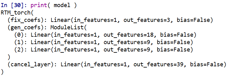
print( model )
######################################################
If you look at the printed out model, it gives a nice summary of the different layers. We have our one layer for the fixed coefficients, and another three sets for our alcohol outlets, 311 calls, and metro entrances. We then have a final cancel layer. The idea behind the final cancel layer is that the variable selection routine in RTM can still end up not selecting any variables for a set. I ended up not using it here though, as it was too aggressive in this example. (So will need to tinker with that some more!)
The variable selection routine is very volatile – so if you have very correlated inputs, you can essentially swap one for the other and get near equivalent predictions. I often see folks who do RTM analyses say something along the lines of, “OK this RTM selected A, and this RTM selected B, so they are different effects in these two samples” (sometimes pre/post, other times comparing different areas, and other times different crime outcomes). I think this is probably wrong though to make that inference, as there is quite a bit of noise in the variable selection process (and the variable selection process itself precludes making inferences on the coefficients themselves).
My deep learning example inherited the same problems. So if you change the initialized weights, it may end up selecting totally different inputs in the end. To get the variable selection routine to at least select the same crime generator variables in my tests, I do a burn in period in which I implement a random dropout scheme. So instead of the typical dropout, for every forward pass it does a random dropout to only select one variable randomly out of each crime generator set. After that converges, I then use a pruning layer to only pick the coefficient that has the largest effect, and again do a large set of iterations to make sure the results converged. So different means but same ends to the typical RTM steps 4 and 5 above. I also have like I said a ReLU transformation after each layer, so the crime generator variables are always positive, any negative effects will be pruned out.
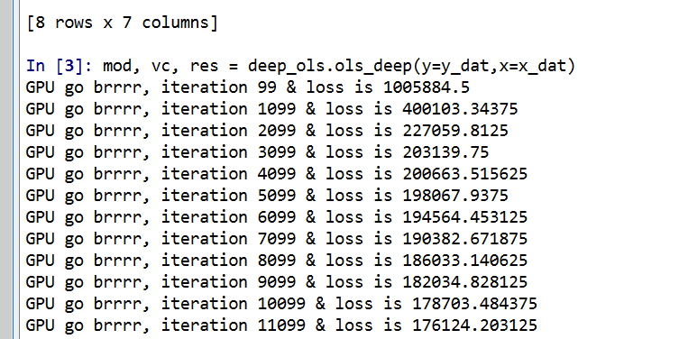
One thing that is nice about deep learning is that it can be quite fast. Here each of these 10,000 iteration sets take less than a minute on my desktop with a GPU. (I’ve been prototyping models with more parameters and more observations at work on my laptop with just a CPU that only take like 10 to 20 minutes).
######################################################
#Burn in part, random dropout
for t in range(10000):
#Forward pass
y_pred = model(x=x_ten)
#Loss
loss_insample = criterion(y_pred, y_ten)
optimizer.zero_grad()
loss_insample.backward(retain_graph=True)
optimizer.step()
if t % 1000 == 0:
print(f'loss: {loss_insample.item()}' )
#Switching to pruning all but the largest effects
model.l1_prune()
for t in range(10000):
#Forward pass
y_pred = model(x=x_ten, mask_type=None, cancel=False)
#Loss
loss_insample = criterion(y_pred, y_ten)
optimizer.zero_grad()
loss_insample.backward(retain_graph=True)
optimizer.step()
if t % 1000 == 0:
print(f'loss: {loss_insample.item()}' )
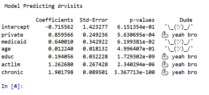
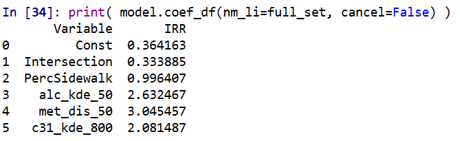
print( model.coef_df(nm_li=full_set, cancel=False) )
######################################################
And this prints out the results (as incident rate ratios), so you can see it selected 50 meters alcohol kernel density, 50 meters distance to the nearest metro station, and kernel density for 311 calls with an 800 meter bandwidth.
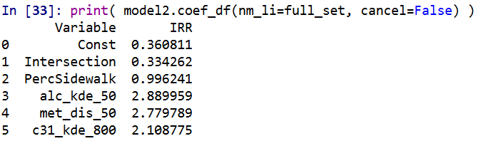
I have in the code another example model when using a different seed. So testing out on around 5 different seeds it always selected these same distance/density variables, but the coefficients are slightly different each time. Here is an example from setting the seed to 12.
These models are nothing to brag about, using the typical z-score the predictions and set the threshold to above 2, the PAI is only around 3 (both for in-sample 2011 and out of sample 2012 is slightly lower). It is a tough prediction task – the mean number of violent crimes per street unit per year is only 0.3. Violent crime is fortunately very rare!
But with only three different risk variables, we can do a quick conjunctive analysis, and look at the areas of overlap.
######################################################
#Adding model 1 predictions back into the dataset
pred_mod1 = pd.Series(model(x=x_ten, mask_type=None, cancel=False).exp().detach().numpy())
crime_data['Pred_M1'] = pred_mod1
#Check out the areas of overlapping risk
mod1_coef = model.coef_df(nm_li=full_set, cancel=False)
risk_vars = list(set(mod1_coef['Variable']) - set(const_li))
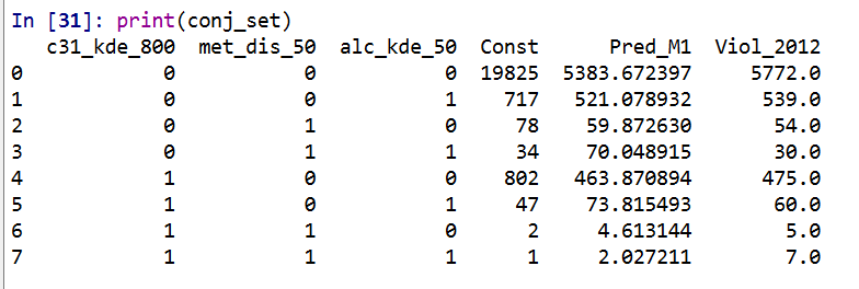
conj_set = crime_data.groupby(risk_vars, as_index=False)['Const','Pred_M1','Viol_2012'].sum()
print(conj_set)
######################################################
In this table Const is the total number of street units selected, Pred_M1 is the expected number of crimes via Model 1, and then I show how well it conforms to the predictions out of sample 2012. So you can see in the aggregate the predictions are not too far off. There only ends up being one street unit that overlaps for all three risk factors in the study area.
I believe the predictions would be better if I included more crime generator variables. But ultimately the nature of how RTM works it trades off accuracy for simple models. Which is fair – it helps to ease the nature of how a police department (or some other entity) responds to the predictions.
But this trade off results in predictions that don’t fare as well compared with more complicated models. For example I show (with Wouter Steenbeek) that random forests do much better than RTM. To make those models more interpretable we did local decompositions for hot spots, so say this hot spot is 30% alcohol outlets, 20% nearby apartments, etc.
So there is no doubt more extensions for RTM you could do in a deep learning framework, but they will likely always result in more complicated and less interpretable models. Also here I don’t think this code will be better than the traditional RTM folks, the only major benefit of this code is it will run faster – minutes instead of overnight for most jobs.