I am at it again on the bail reform stuff. So we have critics of algorithms in-place of bail say that these bail reforms are letting too many people out (see Chicago and NYC). We also have folks on the other side saying such systems are punishing too many people (the Philly piece is more about probation, but the critique applies the same to pre-trial algorithms). So how can risk assessment algorithms both be too harsh and too lenient at the same time? The answer is that how harsh or lenient is not intrinsic to the algorithm itself, people can choose the threshold to be either.

At its most basic, risk assessment algorithms provide an estimate of future risk over some specific time horizon. For example, after scored for a pre-trial risk assessment, the algorithm may say an individual has a 30% probability of committing a crime within the next 3 months. Is 30% low risk, and so they should be released? Or is 30% high risk? The majority of folks do not go on to commit a new offense awaiting for trial, so 30% overall may be really high actually relative to most folks being assessed. So how exactly do you decide the threshold – at what % is it too high and they should be detained pre-trial?

For an individual cost-benefit analysis, you consider the costs of pre-trial detainment (the physical costs to detain a person for a specific set of time, as well as the negative externalities of detention for individuals) vs the cost to society of whether a future crime occurs. So for the 30% mark, say that average crime cost to society is $10,000 (this is ignoring that violent crimes cost more than property crime, in practice you can get individual probability estimates for each and combine them together). So the expected risk if we let this person go would then be $10,000*0.3 = $3,000. Whether the 3k risk is worth the pre-trial detention depends on how exactly we valuate detention. Say we have on average 90 days pre-trial detention, and the cost is something like $200 up front fixed costs plus $50 per day. We would then have a cost to detain this person as $200 + $50*90 = $4,700. From that individual perspective, it is not worth to detain that person pre-trial. This is a simplified example, e.g. this ignores any negative externality cost of detaining (e.g. lost wages for individuals detained), but setting the threshold risk for detaining or releasing on recognizance (ROR) should look something like this.

One of the things I like about this metric is that it places at the forefront how another aspect of bail reform – the time to trial – impacts costs. So if you reduce the time to trial, for those ROR’d you reduce the time horizon of risk. (Those only out 1 month have less time to recidivate than those that have to wait 6 months.) It also reduces the cost of detaining individuals pre-trial as well (costs less for both the state and the individual to only be in jail 1 month vs 6 months). It may be to make everyone happy, we should reduce the queue so we can get people to trial faster. (But in the short term risk assessment tools I think have a great upside to both increase public safety as well as reduce imprisonment costs.)

Evaluating Overall Crime Effects

Part of the reason folks are not happy with the current bail reforms is that they think it is increasing overall crime (see this example in Dallas). Here is an example graph though that folks doing these assessments should be providing, both in terms of up-front establishing the threshold for risk, as well as evaluating the efficacy of the risk assessment tool in practice.

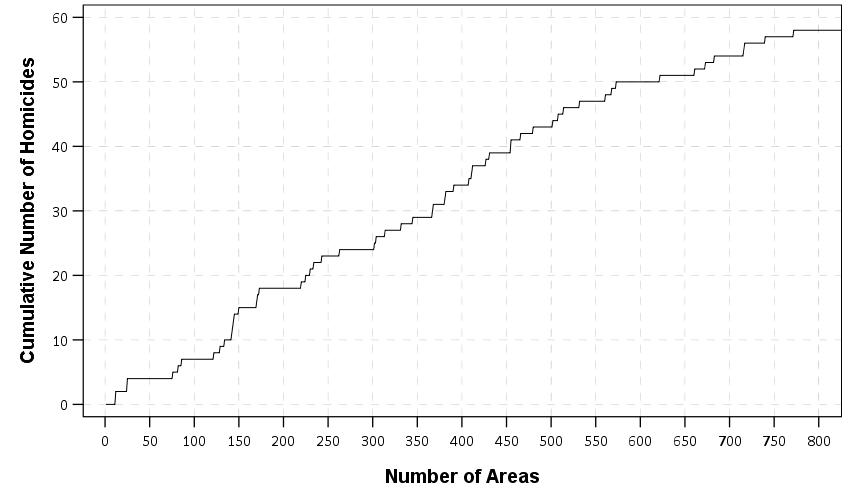
I will use the data from my prior posts on false positives to illustrate. For the graph, you place on the X axis the cumulative number of people that are detained, and the Y axis you place the expected number of crimes that your model thinks will be committed by those folks who are ROR’d. So a simplified table may be

Person %crime
   A     0.5
   B     0.4
   C     0.3
   D     0.2
   E     0.1

If we let all of these folks go, we would expect they commit a total of 1.5 crimes (the sum of the percent predicted crime column) forecasted per our risk assessment algorithm. If we detained just person A, we have 1 in the detain column, and then a cumulative risk for the remaining folks of 1 (the sum of the predicted crime column for those that are remaining and are not detained). So then we go from the above table to this table by increasing the number of folks detained one-by-one.

Detained ExpectedCrimes
   0          1.5
   1          1.0
   2          0.6
   3          0.3
   4          0.1
   5          0

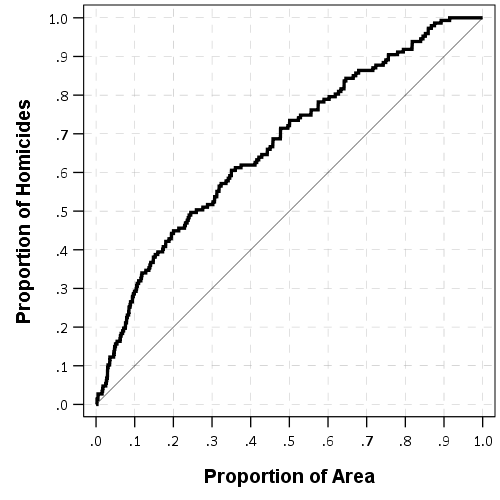
Here is what that graph looks like using the ProPublica data, so if we apply this strategy to the just under 3,000 cases (in my test set from the prior blog post). So you can see that if we decided to detain no-one, we would expect a total of 1,200 extra crimes. And this curve decreases over detaining everyone. So you may say I don’t want more than 200 crimes, which you would need to have detained 1,500 people in the prior example (and happens to result in a risk threshold of 36% in this sample).

Using historical data, this is good to establish a overall amount of crime risk you expect to occur from a particular set of bail reform decisions. To apply it to the future threshold decision making, you need to assume the past in terms of the total number of people arrested as well as the risk distribution stays the same (the latter I don’t think is a big issue, and the former you should be able to make reasonable projections if it is not constant). But this sets up the hypothetical, OK if we release this many more people ROR, we expect this many more crimes to occur as an upfront expectation of bail reform. It may be even if the individual cost-benefit calculation above says release, this would result in a total number of extra crimes folks deem unacceptable when applying that decision to everyone. So we can set the threshold to say we only want 10 extra crimes to happen because of bail reform, or 50 extra, or 100 extra, etc. This example again just aggregates all crime together, but you can do the same thing for every individual crime outcome you are interested in.

After the assessment is in place, this is actually necessary monitoring folks should do be doing anyway to ensure the model is working as expected. That is, you get an estimate of the number of crimes folks who are released you think would commit per your risk assessment model. If you predict more/less than what you see amongst those released, your model is not well calibrated and needs to be updated. In practice you can’t just estimate a predictive model once and then use it forever, you need to constantly monitor whether it is still working well in real life. (Actually I showed in my prior blog post that the model was not very good, so this is a pretty big over-estimate of the number of crimes in this sample.)

This should simultaneously quell complaints about bail reform is causing too many crimes. The lack of this information is causing folks to backlash against these predictive algorithms (although I suspect they do better than human judges, so I suspect they can reduce crime overall if used wisely). Offhand the recent crime increases in Philly, NYC, and Dallas I’m skeptical are tied to these bail reform efforts (they seem too big of increases or too noisy up/downs to reliably pin to just this), but maybe I am underestimating how many people they are letting out and the cumulative overall risk expected from the current models in those places. On the flip-side folks are right to question those Chicago stats, I suspect the risk algorithm should be saying that more crimes are occurring then they observed (ignoring what they should or should not be counting as recidivated).

I’d note these metrics I am suggesting here should be pretty banal to produce in practice. It is administrative data already collected and should be available in various electronic databases. So in practice I don’t know why this data is not readily available in various jurisdictions.

What about False Positives?

One thing you may notice is that in my prior cost-benefit analysis I didn’t take into consideration false positives. Although my prior post details how you would set this, there is a fundamental problem with monitoring false positives (those detained but who would not go on to recidivate) in practice. In practice, you can’t observe this value (you can only estimate it from historical data). Once you detain an individual, by construction they aren’t given the chance to recidivate. So you don’t get any on-policy feedback about false-positives, only false-negatives (folks who were released and went on to commit a crime pre-trial).

This I think puts a pretty big nail in the coffin of using false positive rates as a policy goal for bail reform in practice. Like I said earlier, you can’t just set a model once and expect it to work forever in the future. But, I actually don’t think that should be considered in the cost-benefit calculus anyway. So traditionally people tend to think of setting the threshold for predictive models like this confusion table, where different outcomes in the table have different costs to individuals and to society:

In this table those on the bottom row are those detained pre-trial. So in the hypothetical, you may say if we could someone know the false positives, we should calculate extra harm that pre-trial detainment causes to those individuals (lost wages, losing job, health harms, etc.). But for the folks who would have gone on and recidivated, we should just calculate the bare bones cost of detainment.

I think this is the wrong way to think about it though. Those harms are basically across the board for everyone – even if the person was likely to recidivate they still bear those subsequent harms of being incarcerated. Whether you think people deserve the harm does not make it go away.

The main reason I am harping on bail reform so much (folks who know my work will realize it is outside my specific research area) is that the current bail system is grossly inefficient and unequitable. These are folks that piling on monetary bail costs are the exact wrong way to ensure safety and to promote better outcomes for these folks.

It is a hard decision to make on who to detain vs who to let go. But pretending the current state of judges making these decisions on whatever personal whims they have and thinking we are better off than using a cost-benefit approach and algorithmic assessments is just sticking your head in the sand.