One area of prediction in criminal justice I think has alot of promise is using predictive algorithms in place of bail decisions. So using a predictive instrument to determine whether someone is detained pre-trial based on risk, or released on recognizance if you are low risk. Risk can be either defined as based on future dangerousness or flight risk. This cuts out the middle man of bail, which doesn’t have much evidence of effectiveness, and has negative externalities of placing economic burdens on folks we really don’t want to pile that onto. It is also the case algorithms can likely do quite a bit better than judges in figuring out future risk. So an area I think they can really do good compared to current status quo in the CJ system.

A reasonable critique of such systems though is they can have disparate racial impact. For example, ProPublica had an article on how the Compas risk assessment instrument resulted in more false positives for black than white individuals. Chris Stucchio has a nice breakdown for why this occurs, which is not due to the Compas being intrinsically racist algorithm, but due to the nature of the baseline risks for the two groups.

Consider a very simple example to illustrate. Imagine based on our cost-benefit analysis, we determine the probability threshold to flag a individual as high risk is 60%. Now say our once we apply our predictions, for those above the threshold, whites are all predicted to be 90%, and blacks are all 70%. If our model is well calibrated (which is typically the case), the false positive rate for whites will be 10%, and will be 30% for blacks.

It is actually a pretty trivial problem though to balance false positive rates between different groups, if that is what you want to do. So I figured I would illustrate here using the same ProPublica data. There are trade-offs though with this, balancing false positives means you lose out on other metrics of fairness. In particular, it means you don’t have equality of treatment – different racial groups will have different thresholds. The full data and code I use to illustrate this can be downloaded here.

An Example in Python

To illustrate how we would balance the false positive rates between groups, I use the same ProPublica risk assessment data. So this isn’t per se for bail decisions, but works fine as an illustration. First in python I load my libraries, and then read in the data – it is a few over 11,000 cases.

import pandas as pd
import os
import numpy as np
from sklearn.ensemble import RandomForestClassifier
import matplotlib.pyplot as plt

my_dir = r'C:\Users\andre\Dropbox\Documents\BLOG\BalanceFalsePos'
os.chdir(my_dir)

#For notes on data source, check out 
#https://github.com/apwheele/ResearchDesign/tree/master/Week11_MachineLearning
recid = pd.read_csv('PreppedCompas.csv')
print( recid.head() )

Next I prepare the dataset for modelling. I am not using all of the variables in the dataset. What I predict here is recidivism post 30 days (there are a bunch of recidivism right away in the dataset, so I am not 100% sure those are prior to screening). I use the three different aggregate compas scores, juvenile felony count, whether they were male, how old they were, and whether the current charge to precipitate screening is a felony or misdemeanor. I include the race variable in the dataset, but I won’t be using it in the predictive model. (That point deserves another blog post, contra to what you might expect, leaving race flags in will often result in better outcomes for that protected class.)

#Preparing the variables I want
recid_prep = recid[['Recid30','CompScore.1','CompScore.2','CompScore.3',
                    'juv_fel_count','YearsScreening']]
recid_prep['Male'] = 1*(recid['sex'] == "Male")
recid_prep['Fel'] = 1*(recid['c_charge_degree'] == "F")
recid_prep['Mis'] = 1*(recid['c_charge_degree'] == "M")
recid_prep['race'] = recid['race']
print( recid['race'].value_counts() ) #pretty good sample size for both whites/blacks

Next I make my testing and training sets of data. In practice I can perfectly balance false positives retrospectively. But having a test set is a better representation of reality, where you need to make some decisions on the historical data and apply it forward.

#Now generating train and test set
recid_prep['Train'] = np.random.binomial(1,0.75,len(recid_prep))
recid_train = recid_prep[recid_prep['Train'] == 1]
recid_test = recid_prep[recid_prep['Train'] == 0]

Now the procedure I suggest to balance false-positives doesn’t matter how you generate the predictions, just that we need a predicted probability. Here I use random forests, but you could use whatever machine learning or logistic regression model you want. Second part just generates the predicted probabilities for the training dataset.

#Now estimating the model
ind_vars = ['CompScore.1','CompScore.2','CompScore.3',
            'juv_fel_count','YearsScreening','Male','Fel','Mis'] #no race in model
dep_var = 'Recid30'
rf_mod = RandomForestClassifier(n_estimators=500, random_state=10)
rf_mod.fit(X = recid_train[ind_vars], y = recid_train[dep_var])

#Now getting the predicted probabilities in the training set
pred_prob = rf_mod.predict_proba(recid_train[ind_vars] )
recid_train['prob'] = pred_prob[:,1]
recid_train['prob_min'] = pred_prob[:,0]

Now to balance false positives, I will show a graph. Basically this just sorts the predicted probabilities in descending order for each racial group. Then you can calculate a cumulate false positive rate for different thresholds for each group.

#Making a cusum plot within each racial group for the false positives
recid_train.sort_values(by=['race','prob'], ascending=False, inplace=True)
recid_train['const'] = 1
recid_train['cum_fp'] = recid_train.groupby(['race'])['prob_min'].cumsum()
recid_train['cum_n'] = recid_train.groupby(['race'])['const'].cumsum()
recid_train['cum_fpm'] = recid_train['cum_fp'] / recid_train['cum_n']
white_rt = recid_train[recid_train['race'] == 'Caucasian']
black_rt = recid_train[recid_train['race'] == 'African-American' ] 

And now the fun part (and least in output, not really in writing matplotlib code).

#now make the chart for white and black
fig, ax = plt.subplots()
ax.plot(black_rt['prob'], black_rt['cum_fpm'], drawstyle='steps', color='b', label='Black')
ax.plot(white_rt['prob'], white_rt['cum_fpm'], drawstyle='steps', color='r', label='White')
ax.set_xlim(1, 0)  # decreasing probs
plt.xticks(np.arange(1.0,-0.1,-0.1))
ax.set_xlabel('Predicted Probability')
ax.set_ylabel('Mean False Positive Rate')
ax.grid(True,linestyle='--')
ax.legend(facecolor='white', framealpha=1)
plt.savefig('FP_Rate.png', dpi=2000, bbox_inches='tight')
plt.show()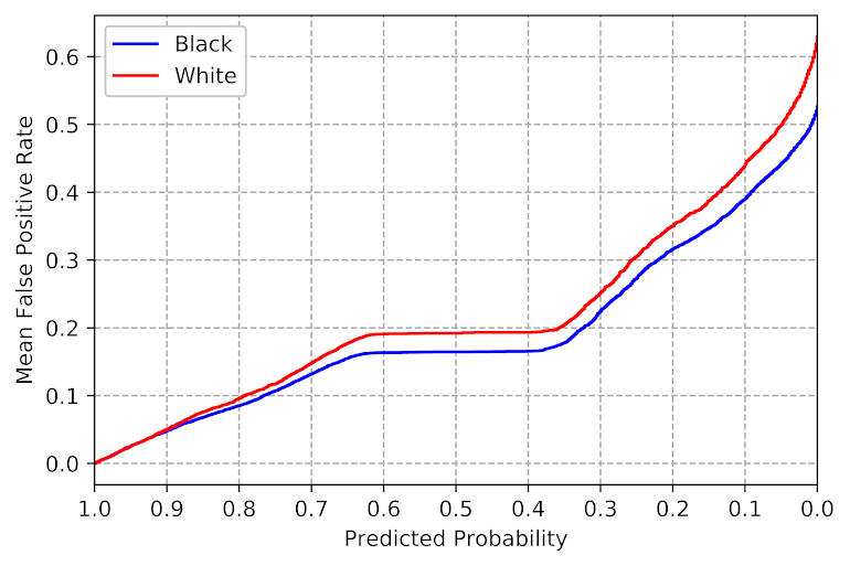

So what this chart shows is that if we set our threshold to a particular predicted probability (X axis), based on the data we would expect a false positive rate (Y axis). Hence if we want to balance false positives, we just figure out the race specific thresholds for each group at a particular Y axis value. Here we can see the white line is actually higher than the black line, so this is reverse ProPublica findings, we would expect whites to have a higher false positive rate than blacks given a consistent predicted probability of high risk threshold. So say we set the threshold at 10% to flag as high risk, we would guess the false positive rate among blacks in this sample should be around 40%, but will be closer to 45% in the white sample.

Technically the lines can cross at one or multiple places, and those are places where you get equality of treatment and equality of outcome. It doesn’t make sense to use that though from a safety standpoint – those crossings can happen at a predicted probability of 99% (so too many false negatives) or 0.1% (too many false positives). So say we wanted to equalize false positive rates at 30% for each group. Here this results in a threshold for whites as high risk of 0.256, and for blacks a threshold of 0.22.

#Figuring out where the threshold is to limit the mean FP rate to 0.3
#For each racial group
white_thresh = white_rt[white_rt['cum_fpm'] > 0.3]['prob'].max()
black_thresh = black_rt[black_rt['cum_fpm'] > 0.3]['prob'].max()
print( white_thresh, black_thresh )

Now for the real test, lets see if my advice actually worked in a new sample of data to balance the false positive rate.

#Now applying out of sample, lets see if this works
pred_prob = rf_mod.predict_proba(recid_test[ind_vars] )
recid_test['prob'] = pred_prob[:,1]
recid_test['prob_min'] = pred_prob[:,0]

white_test = recid_test[recid_test['race'] == 'Caucasian']
black_test = recid_test[recid_test['race'] == 'African-American' ]

white_test['Flag'] = 1*(white_test['prob'] > white_thresh)
black_test['Flag'] = 1*(black_test['prob'] > black_thresh)

white_fp= 1 - white_test[white_test['Flag'] == 1][dep_var].mean()
black_fp = 1 - black_test[black_test['Flag'] == 1][dep_var].mean()
print( white_fp, black_fp )

And we get a false positive rate of 54% for whites (294/547 false positives), and 42% for blacks (411/986) – yikes (since I wanted a 30% FPR). As typical, when applying your model to out of sample data, your predictions are too optimistic. I need to do some more investigation, but I think a better way to get error bars on such thresholds is to do some k-fold metrics and take the worst case scenario, but I need to investigate that some more. The sample sizes here are decent, but there will ultimately be some noise when deploying this in practice. So basically if you see in practice the false positive rates are within a few percentage points that is about as good as you can get in practice I imagine. (And for smaller sample sizes will be more volatile.)