So the other day on Hackernews, a startup had a question in their entry to interview:
You have m mentees – You have M mentors – You have N match scores between mentees and mentors, based on how good of a match they are for mentorship. – mxM > N, because not every mentee is eligible to match with every mentor. It depends on seniority constraints. – Each mentee has a maximum mentor limit of 1 – Each mentor has a maximum mentee limit of l, where 0<l<4 How would you find the ideal set of matches to maximize match scores across all mentees and mentors?
Which I am not interested in applying to this start-up (it is in Canada), but it is a fun little distraction. I would use linear programming to solve this problem – it is akin to an assignment matching problem.
So here to make some simple data, I have two mentors and four mentees. Each mentee has a match score to its mentor, and not all mentees have a match score with each mentor.
# using googles or-tools
from ortools.linear_solver import pywraplp

# Create data
menA = {'a':0.2, 'b':0.4, 'c':0.5}
menB = {'b':0.3, 'c':0.4, 'd':0.5}
So pretend each mentor can be assigned two mentees, what is the optimal pairing? If you do a greedy approach, you might say, for menA lets do the highest, b then c. And then for mentor B, we only have left mentee d. This is a total score of 0.4 + 0.5 + 0.5 = 1.4. If we do greedy the other way, we get mentor B assigned c and d, and then mentor A can have a and b assigned, with a score of 0.4 + 0.5 + 0.4 + 0.2 = 1.5. And this ends up being the optimal approach in this scenario.
Here I am going to walk through creating this model in google’s OR tools package. First we create a few different data structures, one is a set of pairs of mentor/mentees, and these will end up being our decision variables. The other is a set of the unique mentees (and we will need a set of the unique mentors as well) later for the constraints.
# a few different data structures
# for our linear programming problem
dat = {'A':menA,
       'B':menB}

mentees = []

pairs = {}
for m,vals in dat.items():
    for k,v in vals.items():
        mentees.append(k)
        pairs[f'{m},{k}'] = v

mentees = set(mentees)
Now we can create our model, and here we are maximizing the matches. Edit: Note that GLOP is not an MIP solver, leaving the blog post as since in my experiments it does always return 0/1’s (some LP formulations will always return binary, I do not know if this is always true for this one or not). If you want to be sure to use integer variables though, use pywraplp.Solver.CreateSolver("SAT") instead of GLOP.
# Create model, variables
solver = pywraplp.Solver.CreateSolver("GLOP")
matchV = [solver.IntVar(0, 1, p) for p in pairs.keys()]

# set objective, maximize matches
objective = solver.Objective()
for m in matchV:
    objective.SetCoefficient(m, pairs[m.name()])

objective.SetMaximization()
Now we have two sets of constraints. One set is that for each mentor, they are only assigned two individuals. And then for each mentee, they are only assigned one mentor.
# constraints, mentors only get 2
Mentor_constraints = {d:solver.RowConstraint(0, 2, d) for d in dat.keys()}
# mentees only get 1
Mentee_constraints = {m:solver.RowConstraint(0, 1, m) for m in mentees}
for m in matchV:
    mentor,mentee = m.name().split(",")
    Mentor_constraints[mentor].SetCoefficient(m, 1)
    Mentee_constraints[mentee].SetCoefficient(m, 1)
Now we are ready to solve the problem,
# solving the model
status = solver.Solve()
print(objective.Value())

# Printing the results
for m in matchV:
    print(m,m.solution_value())
Which then prints out:
>>> print(objective.Value())
1.5
>>>
>>>
>>> # Printing the results
>>> for m in matchV:
...     print(m,m.solution_value())
...
A,a 1.0
A,b 0.0
A,c 1.0
B,b 1.0
B,c 0.0
B,d 1.0
So here it actually chose a different solution than I listed above, but is also maximizing the match scores at 1.5 total. Mentor A with {a,c} and Mentor B with {b,d}.
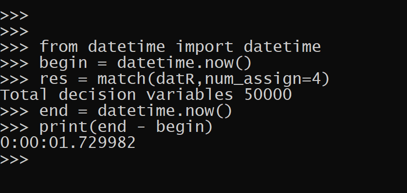
Sometimes people are under the impression that linear programming is only for tiny data problems. Here the problem size grows depending on how filled in the mentor/mentee pairs are. So if you have 1000 mentors, and they each have 50 potential mentees, the total number of decision variables will be 50,000. Which can still be solved quite fast. Note the problem does not per se grow with more mentees per se, since it can be a sparse problem.
To show this a bit easier, here is a function to return the nice matched list:
def match(menDict,num_assign=2):
    # prepping the data
    mentees,mentors,pairs = [],[],{}
    for m,vals in menDict.items():
        for k,v in vals.items():
            mentees.append(str(k))
            mentors.append(str(m))
            pairs[f'{m},{k}'] = v
    mentees,mentors = list(set(mentees)),list(set(mentors))
    print(f'Total decision variables {len(pairs.keys())}')
    # creating the problem
    solver = pywraplp.Solver.CreateSolver("GLOP")
    matchV = [solver.IntVar(0, 1, p) for p in pairs.keys()]
    # set objective, maximize matches
    objective = solver.Objective()
    for m in matchV:
        objective.SetCoefficient(m, pairs[m.name()])
    objective.SetMaximization()
    # constraints, mentors only get num_assign
    Mentor_constraints = {d:solver.RowConstraint(0, num_assign, f'Mentor_{d}') for d in mentors}
    # mentees only get 1 mentor
    Mentee_constraints = {m:solver.RowConstraint(0, 1, f'Mentee_{m}') for m in mentees}
    for m in matchV:
        mentor,mentee = m.name().split(",")
        #print(mentor,mentee)
        Mentor_constraints[mentor].SetCoefficient(m, 1)
        Mentee_constraints[mentee].SetCoefficient(m, 1)
    # solving the model
    status = solver.Solve()
    # figuring out whom is matched
    matches = {m:[] for m in mentors}
    for m in matchV:
        if m.solution_value() > 0.001:
            mentor, mentee = m.name().split(",")
            matches[mentor].append(mentee)
    return matches
I have the num_assigned as a constant for all mentors, but it could be variable as well. So here is an example with around 50k decision variables:
# Now lets do a much larger problem
from random import seed, random, sample
seed(10)
mentors = list(range(1000))
mentees = list(range(4000))

# choose random 50 mentees
# and give random weights
datR = {}
for m in mentors:
    sa = sample(mentees,k=50)
    datR[m] = {s:random() for s in sa}

# This still takes just a few seconds on my machine
# 50k decision variables
res = match(datR,num_assign=4)
And this takes less than 2 seconds on my desktop, which much of that is probably setting up the problem.
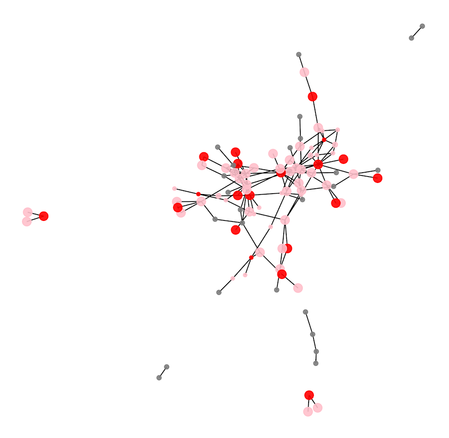
For very big problems, you can separate out the network into connected components, and then run the linear program on each seperate component. Only in the case with dense and totally connected networks will you need to worry much about running out of memory I suspect.
So I have written in the past how I stopped doing homework assignments for interviews. More recently at work we give basic pair coding sessions – something like a python hello world problem, and then a SQL question that requires knowing GROUP BY. If they get that far (many people who say they have years of data science experience fail at those two), we then go onto making environments, git, and describing some machine learning methods.
You would be surprised how many data scientists I interview only know how to code in Jupyter notebooks and cannot do a hello world program from the command line. It is part of the reason I am writing my intro python book. Check out the table of contents and first few chapters below. Only one more final chapter on an end-to-end project before the book will be released on Amazon. (So this is close to the last opportunity to purchase as the lower price before then.)


 Please advise. Thanks!