Wendy Jang, my former student at UTD and now Data Scientist for the Stanislaus County Sheriff’s Dept. writes in:

Hello Andy,

I have some questions about your posting in GitHub. Honestly, I am not good at Python at all. I was playing with your python code and trying to understand the work flow. Then, I can pretty much mimic what you did; however, I encountered some errors along the way.

I was able to follow through lines but then I am stuck on PMed function. Do you know what possibly caused this error? See the screenshot below. Please advise. Thanks!

Specifically, Wendy is asking about my patrol redistricting example with workload inequality constraints. Wendy’s problem here is specifically she likely does not have CPLEX installed. CPLEX is free for academics, but unfortunately costs a bit of money for anyone else (not sure if they have cheaper licensing for public sector, looks like currently about $200 a month).

This was a good opportunity to update some of my code, so now see the two .py files in the DataCreated folder, in particular 01_pmed_class.py has a nice class function. I have additionally added in functionality to create a map, and more importantly eliminate subtours (my solution can potentially return disconnected areas). I have also added the ability to use different solvers.

For this problem CPLEX just works much better (takes around 10 minutes), but I was able to get the SCIP solver to return the same solution in around 5 hours. GLPK did not return a solution even letting it churn out for over 12 hours. I tested CBC for shorter time periods, but that appears to be a no-go as well.

So just a brief overview, the libraries I will be using (check out the end of the post for setting up the conda environment):

import pickle
import pulp
import networkx
import pandas as pd
from datetime import datetime
import matplotlib.pyplot as plt
import geopandas as gpd

class pmed():
    """
    Ar - list of areas in model
    Di - distance dictionary organized Di[a1][a2] gives the distance between areas a1 and a2
    Co - contiguity dictionary organized Co[a1] gives all the contiguous neighbors of a1 in a list
    Ca - dictionary of total number of calls, Ca[a1] gives calls in area a1
    Ta - integer number of areas to create
    In - float inequality constraint
    Th - float distance threshold to make a decision variables
    """
    def __init__(self,Ar,Di,Co,Ca,Ta,In,Th):

I do not copy-paste the entire pmed class in the blog post. It is long, but is the rewrite of my model from the paper. Next, to load in the objects I need to fit the model (which were created/pickled in the 00_PrepareData.py file).

# Loading in data
data_loc = r'D:\Dropbox\Dropbox\PublicCode_Git\PatrolRedistrict\PatrolRedistrict\DataCreated\fin_obj.pkl'
areas, dist_dict, cont_dict, call_dict, nid_invmap, MergeData = pickle.load(open(data_loc,"rb"))

# shapefile for reporting areas
carr_report = gpd.read_file(r'D:\Dropbox\Dropbox\PublicCode_Git\PatrolRedistrict\PatrolRedistrict\DataOrig\ReportingAreas.shp')

And now we can create a pmed object, which has all the info necessary, and gives us a print out of the total number of decision variables and constraints.

# Creating pmed object
pmed12 = pmed(Ar=areas,Di=dist_dict,Co=cont_dict,Ca=call_dict,Ta=12,In=0.1,Th=10)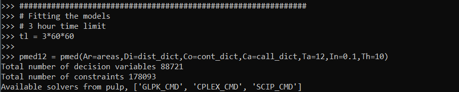

Writing the class this way allows the user to input their own solver, and you can see it prints out the available solvers on your current machine. So to pass in the SCIOPT solver you could do pmed12.solve(solver=pulp.SCIP_CMD()), which again for this problem does find the solution, but takes 5 hours. So here I still stick with CPLEX to just illustrate the new classes functionality:

pmed12.solve(solver=pulp.CPLEX(timeLimit=30*60,msg=True))     # takes around 10 minutes

This prints out a ton of information at the command line that you do not get if you run from within Jupyter notebooks. So for debugging that is much more useful. timeLimit is in seconds, but does not include the presolve phase I believe, so some of these solvers can just get stuck on the presolve forever.

We can look at the results in a nice map if you do have geopandas installed and pass it a geopandas data frame and the key to match it on:

pmed12.map_plot(carr_report, 'PDGrid')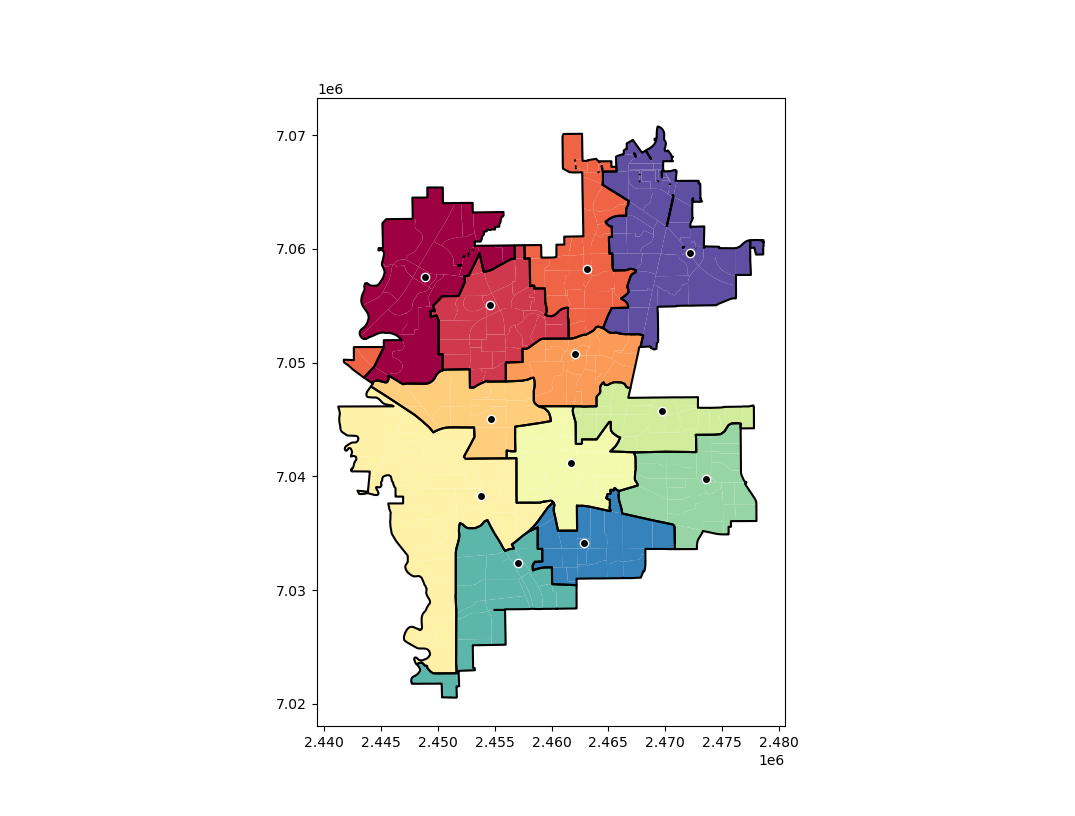

This map shows the new areas and different colors with a thick border, and the source area as a dot with a white outline. So here you can see that we end up having one disconnected area – a subtour in optimization parlance. I have added some methods to deal with this though:

stres = pmed12.collect_subtours()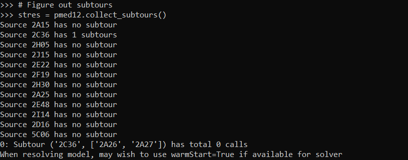

And you can see that for one of our areas it identified a subtour. I haven’t written this to automatically resolve for subtours due to the potential length of the solving time. So here we can see the subtours have 0 calls in them. You can assign those areas to wherever and it does not change the objective function. So that is what I did in the paper and showed how in the Jupyter notebook at the main page for the github project.

So if you are using a function that takes 5 hours, I would suggest you manually fix these subtours if there is an obvious to the human eye easy solution. But here with the shorter solve time with CPLEX I can rerun the algorithm with a warm start, and it runs even faster (under 5 minutes). The .collect_subtours() method adds subtour constraints into the pulp model, so you just need to redo the solve() method to eliminate that particular subtour (I do not know if this is guaranteed to converge though for all problems).

So here in this data eliminating that one subtour results in a solution with no subtours:

pmed12.solve(solver=pulp.CPLEX_CMD(msg=False,warmStart=True))
stres = pmed12.collect_subtours()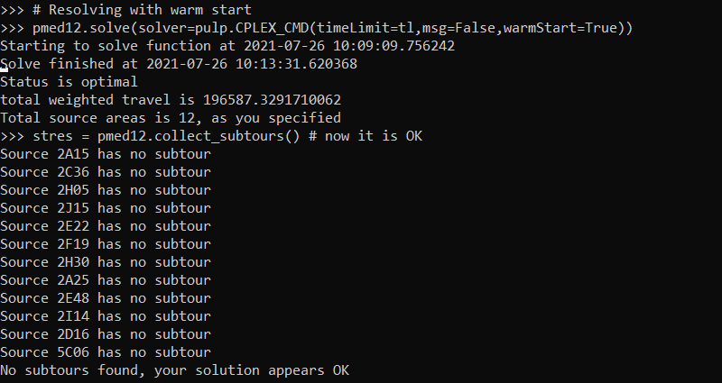

And we can replot the result, which shows it chooses the areas that you would have assigned by eye anyway:

pmed12.map_plot(carr_report, 'PDGrid')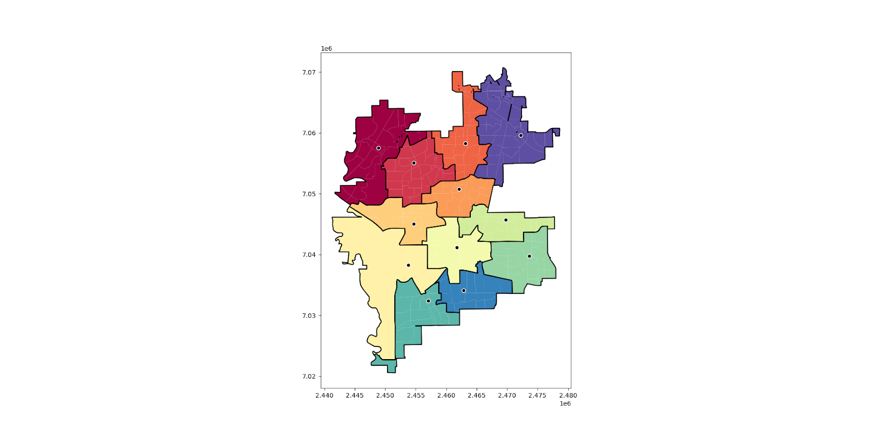

So again for this problem if you have CPLEX I would recommend it (have not tried Gurobi). But at least for this particular dataset SCIOPT was able to solve the problem in 5 hours. So if you are a crime analyst or someone else without academic access to CPLEX you can install the sciopt solver and give that a go for your actual data.

Note that this is based off of results for 325 subareas. So if you have more subareas it will take a longer (and if you have fewer it may be quite a bit shorter).

Setting up the Conda environment

So once you have python installed, you can typically do something like:

pip install pulp

Or via conda:

conda install pyscipopt

I often have trouble though, especially when working with the python geospatial libraries, to install geopandas, fiona, etc. So here what I do is create a new conda environment:

conda create -n linprog
conda activate linprog
conda install -c conda-forge python=3 pip pandas numpy networkx scikit-learn dbfread geopandas glpk pyscipopt pulp

And then you can run the pmedian code above in this environment. I suppose I should turn this into a python package, and I see a bunch of folks anymore are doing docker images as well with their packages in complicated environments. This is actually not that bad, minus geopandas makes things a bit tricky.