New working paper: Choosing Representatives to Deliver the Message in a Group Violence Intervention

I have a new preprint up on SSRN, Choosing Representatives to Deliver the Message in a Group Violence Intervention. This is what I will be presenting at ACJS next Friday the 24th. Here is the abstract:

Objectives: The group based violence intervention model is predicated on the assumption that individuals who are delivered the deterrence message spread the message to the remaining group members. We focus on the problem of who should be given the initial message to maximize the reach of the message within the group.

Methods: We use social network analysis to create an algorithm to prioritize individuals to deliver the message. Using a sample of twelve gangs in four different cities, we identify the number of members in the dominant set. The edges in the gang networks are defined by being arrested or stopped together in the prior three years. In eight of the gangs we calculate the reach of observed call-ins, and compare these with the sets defined by our algorithm. In four of the gangs we calculate the reach for a strategy that only calls-in members under supervision.

Results: The message only needs to be delivered to around 1/3 of the members to reach 100% of the group. Using simulations we show our algorithm identifies the minimal dominant set in the majority of networks. The observed call-ins were often inefficient, and those under supervision could be prioritized more effectively.

Conclusions: Group based strategies should monitor their potential reach based on who has been given the message. While only calling-in those under supervision can reach a large proportion of the gang, delivering the message to those not under supervision will likely be needed to reach 100% of the group.

And here is an image of the observed reach for one of the gang networks using both call-ins and custom notifications.

The paper has the gang networks available at this link, and uses Python to do the network analysis and SPSS to draw the graphs.

If you are interested in applying this to your work let me know! Not only do I think this is a good idea for focused deterrence initiatives for criminal justice agencies, but I think the idea can be more widely applied to other fields in social sciences, such as public health (needle clean/dirty exchange programs) or organizational studies (finding good leaders in an organization to spread a message).

Making and Exploring Crime Networks (Access and Excel)

I’ve been doing quite a bit of stuff with gang networks lately at work. Networks are a total PIA though to create and do data manipulation on in traditional spreadsheets and statistic tools, so I figured I would blog about some of my attempts to ease the pain for fellow crime analysts.

First I will show how to create an edge list in Access from the way a traditional police RMS database is set up. Second I will show a trick about exploring people and gangs by creating a dynamic lookup in Excel. You can download the Access Database I used and the Excel spreadsheet here to follow along.

Making an Edge List in Access

I’ve previously shown how to make an edgelist in SPSS. I’ll cast the net wider and show how to do this in Access though.

In a nutshell, an edge list is a table of the form:

Person A, Person B
Person B, Person C
Person C, Person D

Where being in the same row shows some type of connection between the two persons, e.g. Person A is connected to Person B. In police databases the connections most often of interest are co-offending (e.g. two people were arrested for the same incident) or being stopped together (e.g. in the same car or during the same field interrogation).

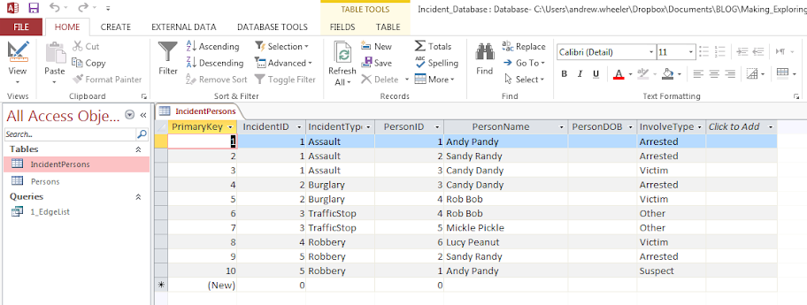
Typically police databases will have a table that lists a common incident identifier, along with persons associated with that incident and their involvement. Here is a screen shot of the simple example I made in an Access Database to mimic this which I named IncidentPersons:

So here we can see that for incident 1, Andy Pandy, Sandy Randy, and Candy Dandy are all persons involved. Candy is the victim, and the other two were arrested. This table is always called something different for every PD’s RMS system, but some examples I have come across are crossref and person_exploded. All RMS’s I have seen though have some sort of table like this.

To make an edge list from this table takes some knowledge of SQL, but it can be done in one query. Basically we will be joining a table to itself, and selecting out distinct rows. Here is the most basic SQL query in Access to accomplish this.

SELECT DISTINCT F.PersonID, F.PersonName, S.PersonID, S.PersonName
FROM IncidentPersons AS F INNER JOIN IncidentPersons AS S ON F.IncidentID = S.IncidentID
WHERE F.PersonID < S.PersonID;

To walk through this, we make two table aliases from the same original IncidentPersons table, F and S. Then we do an INNER JOIN based on the original incident ID. If we stopped here without the last WHERE clase, what would happen is we would have pairs of people with themselves, and with duplicate ties of the form A -> B and B -> A. So selecting only instances in which F.PersonID < S.PersonID eliminates those self edges and duplicates. The last part here is SELECT DISTINCT instead of select. This will make it so any particular edge is only returned once. (If you deleted DISTINCT in this database, Andy Pandy -> Sandy Randy would be returned twice.)

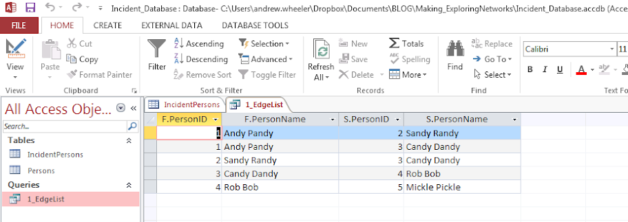
Running this query we then have:

In practice it will be more complicated because you will want to filter certain connections and add more info. on people into the final edge list. Here I ignore the involvement type, but you may want to only restrict matches to certain co-involvements (since offender-victim is of a different nature than co-offending). You also may want to not just know those connected, but count up the number of times those people are connected. For my work, I have always just limited to co-offending and being stopped together (and haven’t ever worried about the number of ties).

Also depending on how the database is normalized, often people names will change/have spelling errors, but they will still be linked to the same personid. These different spellings would cause the DISTINCT selection to not work as expected. A workaround is to only select based on the unique PersonID’s and not import other data, then in an additoional query merge in the person data. For gang network analysis you will likely want to merge in gang affiliation (which will probably be in a seperate table, not in the RMS). If you are still following along though you can figure that stuff out on your own.

Making an Edge Lookup Table in Excel

So now that I have shown how to make the edge table, what to do with it now? (No excuses – since I gave examples in both SPSS and SQL!) Here I will show a simple trick to explore the network using filtering in Excel.

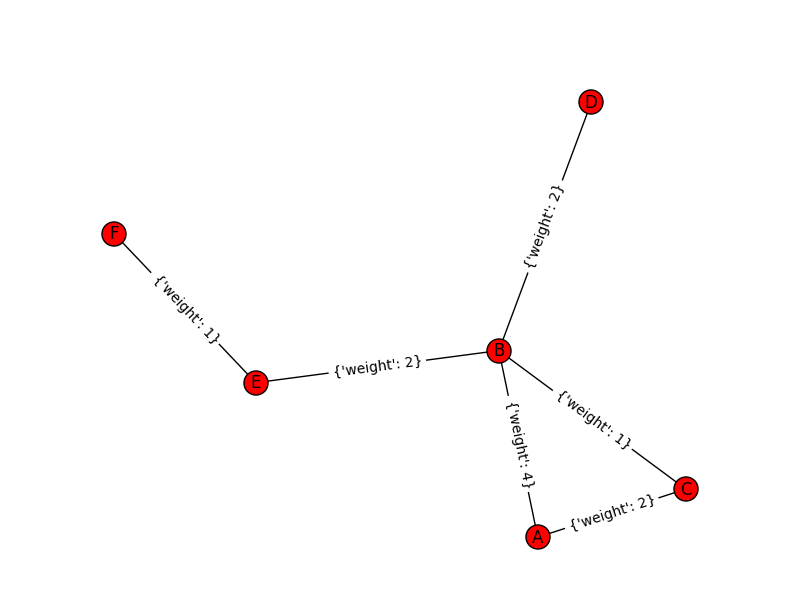
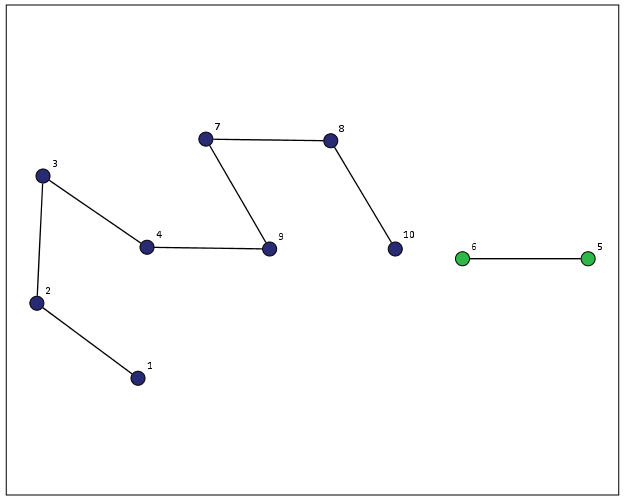
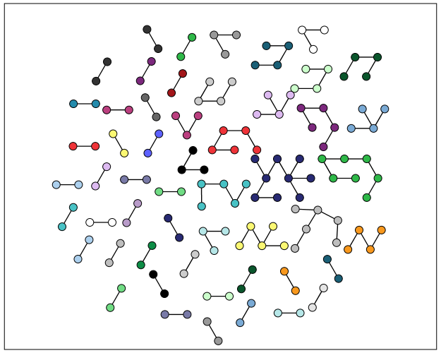
The edge list itself is often the needed format to import into other network based software. So you can make a nice network graph using Gephi or whatever. The graph is good to see the overall form of the network when the graph is limited to only a few nodes, but they are typically really complicated, and tools like Gephi aren’t very good for drilling down into specific people. Here I will show my simple drilldown solution using Excel.

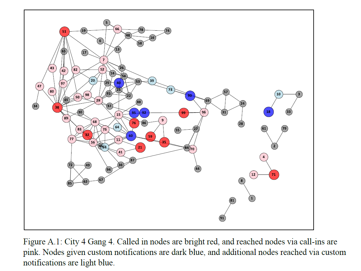
The network I use for this example is entirely made up; it was simulated using NetworkX (python), names are random based on some internet lists of popular baby names and last names I forgot the source of already, and Date of births are random between 1975 and 1997. I also made up a list of 7 gangs (but people have a 9/16 chance to be assigned to no gang).

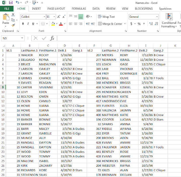
So starting with an edgelist, here is a screenshot of my made up edge list excel table.

The problem in this format is if I filter the Id.1 column for 19 (BONNIE BARKER), they could potentially be in the Id.2 column as well, so I potentially miss edges. A simple solution to this is just to duplicate the data, but switch the order of the edges. Then when I filter by Id = 19, I will get all possible Bonnie Barker edges.

For a simple example of how to do this on a small table, if you start with:

17,19
18,19
19,20
19,21

If you filter the first column by 19, you will eliminate the 19’s in the second column. So just make a new table that has the ID’s reversed:

19,17
19,18
20,19
21,19

And then stack the two tables on top of one another

17,19 |
18,19 |  Table 1
19,20 |
19,21 |
19,17 +
19,18 +  Table 2
20,19 +
21,19 +

So now if you filter the first column by 19 you get 19’s all four connections. This is just three copy-pastes in excel to go from the original edge list to this table.

Now we can make a filter that dynamically changes based on user input. Here I make a selection in the top row, in N2 you can put in a persons ID. Then in A2, the formula is =IF(B2=$N$1,1,0). You can then paste this formula down, and it always references cell N2 because of the absolute $ modifiers.

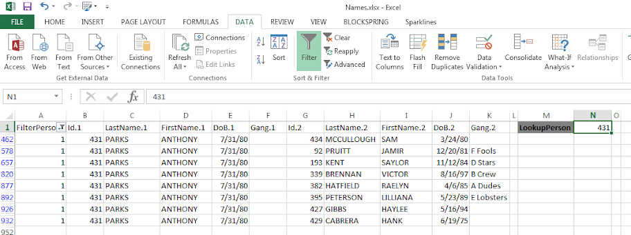
Here is a screenshot of my example LookupTable in excel filtering for person 431.

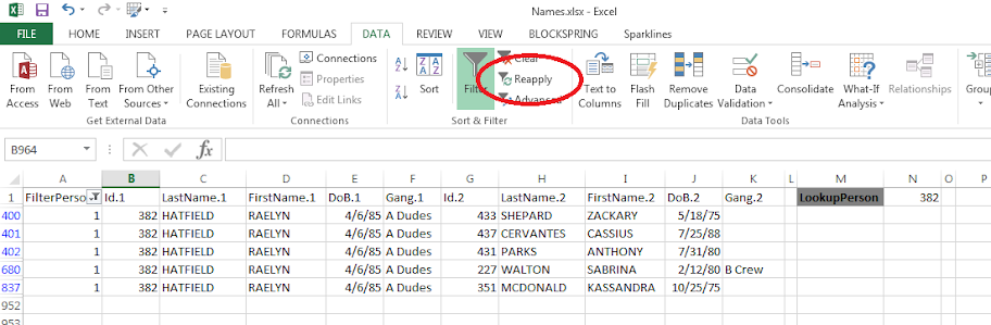
If you update the personid in N1, then hit the reapply button in the toolbar (or hit Ctrl+Alt+L) to update the filter. Here I updated to be person 382.

The context of why I created this example was to identify people that were connected to gang members, but themselves were not in the gang. Basically have a list to take to officers and say, are you sure this person is not an actual member of the gang? The spreadsheet is then a tool if I have a meeting, where someone can say, who is Raelyn Hatfield connected to? I can easily update the id and filter.

You can do this drill down in the original edge table if you have the IF condition look in both the first and second id column, but I do this because it is easier to see who a person is connected to. You only have to look in one column – you don’t have to scan back and forth between two columns to see the connections.

You can also do other aggregations on this table as well. For instance if you aggregate using a pivot table and count the number of instances it is the edge centrality of a person (i.e. the number of different people a person is connected to).

If you want to do a drilldown of specific gangs you could use the same logic and build another filter column, but this will duplicate people when they are connected to another person in the same gang. That would be an instance where it might be easier to use just the original edge table.

Using local Python objects in SPSSINC TRANS – examples with network statistics

When using SPSSINC TRANS, you have a wider array of functions to compute on cases in SPSS. Within the local session, you can create your own python functions within a BEGIN PROGRAM and END PROGRAM block. In SPSSINC TRANS you pass in the values in the current dataset, but you can also create functions that use data in the local python environment as well. An example use case follows in which you create a network in the local python environment using SPSS data, and then calculate several network statistics on the nodes. Here is a simple hierarchical network dataset that signifies managers and subordinates in an agency.

*Edge list. 
DATA LIST FREE / Man Sub (2F1.0). 
BEGIN DATA 
1 2 
2 3 
2 4 
3 5 
3 6 
4 7 
4 8 
END DATA. 
DATASET NAME Boss. 

We can subsequently turn this into a NetworkX graph with the code below. Some of my prior SPSS examples using NetworkX had a bit more complicated code using loops and turning the SPSS dataset into the network object. But actually the way SPSS dumps the data in python (as a tuples nested within a list) is how the add_edges_from function expects it in NetworkX, so no looping required (and it automatically creates the nodes list from the edge data).

BEGIN PROGRAM Python. 
import networkx as nx
import spss, spssdata

alldata = spssdata.Spssdata().fetchall()  #get SPSS data
G = nx.DiGraph()                          #create empty graph
G.add_edges_from(alldata)                 #add edges into graph
print G.nodes()
END PROGRAM.

Note now that we have the graph object G in the local python environment for this particular SPSS session. We can then make our own functions that references G, but takes other inputs. Here I have examples for the geodesic distance between two nodes, closeness and degree centrality, and the average degree of the neighbors.

BEGIN PROGRAM Python.
#path distance
def geo_dist(source,target): 
  return nx.shortest_path_length(G,source,target)
#closeness centrality
def close_cent(v):
  return nx.closeness_centrality(G,v)
#degree
def deg(v):
  return G.degree(v)
#average degree of neighbors
def avg_neideg(v):
  return nx.average_neighbor_degree(G,nodes=[v])[v]
END PROGRAM.

Here is the node list in a second SPSS dataset that we will calculate the mentioned statistics on. For large graphs, this is nice because you can select out a smaller subset of nodes and only worry about the calculations on that subset. For a crime analysis example, I may be monitoring a particular set of chronic offenders, and I want to calculate how close every arrested person within the month is to the set of chronic offenders.

DATA LIST FREE / Employ (F1.0). 
BEGIN DATA 
1 
2
3
4
5
6
7
8
END DATA. 
DATASET NAME Emp. 
DATASET ACTIVATE Emp.

Now we have all the necessary ingredients to calculate our network statistics on these nodes. Here are examples of using SPSSINC TRANS to calculate the network statistics in the local SPSS dataset.

*Geodesic distance from 1.
SPSSINC TRANS RESULT=Dist TYPE=0
  /FORMULA "geo_dist(source=1.0,target=Employ)".

*closeness centrality.
SPSSINC TRANS RESULT=Cent TYPE=0
  /FORMULA "close_cent(v=Employ)".

*degree.
SPSSINC TRANS RESULT=Deg TYPE=0
  /FORMULA "deg(v=Employ)".

*Average neighbor degree.
SPSSINC TRANS RESULT=NeighDeg TYPE=0
  /FORMULA "avg_neideg(v=Employ)".

Laplacian Centrality in NetworkX (Python)

The other day I read a few papers on a new algorithm for calculating centrality in networks. Below are the two papers describing the Laplacian Centrality metric. The first is for non-weighted networks, and the second for weighted networks.

  • Qi, X., Duval, R. D., Christensen, K., Fuller, E., Spahiu, A., Wu, Q., Wu, Y., Tang, W., and Zhang, C. (2013). Terrorist networks, network energy and node removal: A new measure of centrality based on laplacian energy. Social Networking, 02(01):19-31.
  • Qi, X., Fuller, E., Wu, Q., Wu, Y., and Zhang, C.-Q. (2012). Laplacian centrality: A new centrality measure for weighted networks. Information Sciences, 194:240-253. PDF Here.

The metric is fairly intuitive I think. The centrality parameter is a function of the local degree plus the degree’s of the neighbors (with different weights for each). I figured it would be a quick programming exercise (which means I spent way too long trying to implement it!). To follow is some code that replicates the measures for both weighted and non-weighted graphs, using the Python networkx library.

The non-weighted graph code is easy, and is a near copy-paste from some igraph code snippet that was already available. Just some updates to idiom’s for NetworkX specifically. The norm option specifies whether you want solely the numerator value, the difference between the energy in the full graph versus the graph with the node removed (norm=False), or whether you want to divide this value by the energy for the full graph. Note this function ignores the weights in the graph. nbunch is if you want to pass the function only a subset of points to calculate the centrality. (If you do that you might as well have norm=False for time savings as well.)

def lap_cent(graph, nbunch=None, norm=False):
  if nbunch is None:
    vs = graph.nodes()
  else:
    vs = nbunch
  degrees = graph.degree(weight=None)
  if norm is True:
    den = sum(v**2 + v for i,v in degrees.items())
    den = float(den)
  else:
    den = 1
  result = []
  for v in vs:
    neis = graph.neighbors(v)
    loc = degrees[v]
    nei = 2*sum(degrees[i] for i in neis)
    val = (loc**2 + loc + nei)/den
    result.append(val)
  return result

The weighted network is a bit more tricky though. I thought coding all of the two walks seemed a royal pain, so I developed a different algorithm that I believe is quicker. Here are three functions, but the last one is the one of interest, lap_cent_weighted. The options are similar to the unweighted version, with the exception that you can pass a weight attribute (which is by default named ‘weight’ in NetworkX graphs).

def lap_energy(graph, weight='weight'):
  degrees = graph.degree(weight=weight)
  d1 = sum(v**2 for i,v in degrees.items())
  wl = 0
  for i in graph.edges(data=True):
    wl += (i[2].get(weight))**2
  return [d1,2*wl]

def cw(graph,node,weight='weight'):
  neis = graph.neighbors(node)
  ne = graph[node]
  cw,sub = 0,0
  for i in neis:
    we = ne[i].get(weight)
    od = graph.degree(i,weight=weight)
    sub += -od**2 + (od - we)**2
    cw += we**2
  return [cw,sub]

def lap_cent_weighted(graph, nbunch=None, norm=False, weight='weight'):
  if nbunch is None:
    vs = graph.nodes()
  else:
    vs = nbunch
  if norm == True:
    fe = lap_energy(graph,weight=weight)
    den = float(fe[0]+fe[1])
  else:
    den = 1
  result = []
  for i in vs:
     d2 = graph.degree(i,weight=weight)
     w2 = cw(graph,i,weight=weight)
     fin = d2**2 - w2[1] + 2*w2[0]
     result.append(fin/den)
  return result

For a brief overview of the new algorithm (in some quick and dirty text math), to define the energy of the entire graph it is:

sum(di^2) + 2*sum(wij^2)   (1)

Where di are the degrees for all i nodes, and the second term is 2 times the sum of the weights squared. So when you take out a particular node, say ‘A’, the drop in the second term is easy, just iterate over the neighbors of ‘A’, and calculate 2*sum(waj^2), then subtract that from the second term in equation 1.

The first term is slightly more complex. First there is a decrease due to simply the degree of the removed node, da^2. There is also a decrease in the degree on the neighboring nodes as well, so you need to calculate their updated contribution. The necessary info. is available when you iterate over the neighbor list though, and if the original contribution is di^2, and the weight of wia, then the updated weight is -di^2 + (di - wia)^2. You can calculate this term at the same time you calculate the decrease in the weights in the second term.

I believe this algorithm is faster than the one originally written in the second paper. It should be something like O(n*a), where a is the average number of neighbors for the entire graph, and n are the number of nodes. Or in worst case a is the maximum number of neighbors any node has in the graph (which should be less than or equal to the max degree in a weighted graph).

Here is an example of using the functions with the small, toy example in the weighted network paper. Note that the lap_cent function ignores the weights.

import networkx as nx

Gp = nx.Graph()
ed = [('A','B',4),('A','C',2),('C','B',1),('B','D',2),('B','E',2),('E','F',1)]
Gp.add_weighted_edges_from(ed)

x = lap_cent(Gp)
xw = lap_cent_weighted(Gp, norm=True)
for a,b,c in zip(Gp.nodes(),x,xw):
  print a,b,c

Which prints out at the console:

A 18 0.7 
C 18 0.28 
B 34 0.9 
E 16 0.26 
D 10 0.22 
F 6 0.04

If you want to see that the graph is the same as the graph in the weighted Qi paper, use below.

import matplotlib.pyplot as plt
pos=nx.spring_layout(Gp) # positions for all nodes
nx.draw(Gp,pos=pos)
nx.draw_networkx_labels(Gp,pos=pos)
nx.draw_networkx_edge_labels(Gp,pos=pos)
plt.show()

Presentation at IACA 2015: An Exploratory Network Analysis of Hot People and Places

My work was accepted at the 2015 International Association of Crime Analysts Conference, so I will be going to Denver this fall to present. These are "NIJ Research Track" presentations, but basically took the place of the old MAPS conference presentations. So on Thursday at 2:30 (Panel 9) I will be presenting. The title of the presentation is An Exploratory Network Analysis of Hot People and Places, and below is the abstract for the talk:

Intelligence led policing practices focus on chronic offenders and hot spots of crime. I examine the connections between these hot people and hot places by considering micro places (street segments and intersections) and people as nodes in an interconnected network. I focus on whether hot people tend to have a finite set of locations they congregate, and whether hot places have unique profiles of chronic offenders. The end goal is to identify if observed patterns can help police combine targeted enforcement of hot people and hot places in one overarching strategy.

This is still a work in progress, but here is a quick preview. This graph is a random sample of offender footprints in each panel.

Also during this slot there are two other presentations, below is their info:

Title: Offender Based Investigations: A Paradigm Shift in Policing, Author: Chief James W. Buie, Gaston County Police

Abstract: Routine activity theory and research conducted by Wiles, P & Costello, A. (2000) ‘The Road to Nowhere’ prove criminals 1) commit crimes where comfortable and 2) are very likely to re-offend. Therefore it makes sense to elevate the importance of offender locations in relation to crimes. Our focus on the offender is called Offender Based Investigations (OBI). We’re using GIS to plot not only crimes but criminals as well. Our experience over the past seven years of utilizing OBI has proven that mapping offenders plays a critical role in solving crimes.

Title: A Spatial Network Analysis of Gangs Author: Davin Hall, Crime Analysis Specialist for the Greensboro PD

Abstract: Gangs are characterized by the associations between members and the territory that members operate in. Many representations of gang territory and gang networks are separate from one another; a map shows the territory while a network map shows linkages between individuals. This presentation demonstrates the combination of territory and network within a single map, for both gangs and gang members. This analysis shows law enforcement a clearer picture of the complex relationships that occur between and within gangs.

You can see the full agenda here. I really enjoyed the presentations last year at Seattle, and this year looks great as well. If you want any more info. on my particular work feel free to send me an email, or if you want to get together at Denver this fall.

Some more on Network distances vs Geographic distances intra-city

A prior post on analyzing distances looked at geographic versus network (road) distances between zip codes in New York and one particular location. Over the large distances the correlation ended up being 0.99. But most crime analysis applications will be within one city, so restricting the distances there will the correlation be just as high? I conducted some analysis in Albany, NY to see if this was the case.

First I took a set of 2,640 street segments and intersections in Albany, defined as basically having over 1 reported crime between 2000 through 2013. (This is a pretty good proxy for places where people are actually located in the city, so places where people might actually travel from/to.) Here is a map of those points showing the coverage.

I then made the 2,640^2 pairs, and then took a random sample of 2,300 of those pairs to calculate the geographic versus the network distance (calculating the network distance using the google distance API). Here is a flow map, again showing it has pretty good coverage of the city.

In this sample the correlation between the network distance and the geographic distance is 0.94, and below is the scatterplot. The red line is the line of equality, so we can see the network distance is always larger.

Making the graph on log scales basically takes away the heteroscedasticity, and shows some short distance outliers.

I then fit a regression of equation of log(Network Distance) ~ Intercept + b_0*log(Geo Distance), and then calculate the studentized residuals. Here is a small multiple flow map of those locations categorized by the truncated studentized residuals. I plotted flows under 200 meters as a red dot, as otherwise they basically have no area on the map to visualize. There are a few notable patterns, the -1 residuals (so closer network and geo distances) are locations along what looks like Central, Washington, Western and New Scotland (running east-west) and Broadway/Pearl (running north-south). So basically straight, major thoroughfares.

It is probable that if more locations in the isthmus and the south western part of the city were selected the distances would be not so nice, but the isthmus itself is largely the Pine Bush park, and the south western part is on the periphery of residential neighborhoods. Exporting the high residuals, what happens in the google distance API is that they are short trips on one way streets, and the to and from and going against the one way. I will have to investigate if you can set the google API to use walking distances to ignore this (as this wasn’t intended as a directed flow like that). Or just learn how to use the CrimeStat or network analysis in ArcMap distance calculation tools!

So although using network distances consistently increases the distances between points, they are still highly correlated, even for shorter in city patterns. If I fixed the flows going against one way streets it would likely be an even higher correlation.

Finding subgroups in a graph using NetworkX and SPSS

This is a task I’ve have to conduct under several guises in the past. Given a set of edges, reduce those edges into unique subgroups based on the transitive closure of those edges. That is, find a group in which all nodes can reach one another (via however many steps are necessary) but are completely separated from all other nodes.

This is steeped in some network language jargon, so I will give a few examples in data analysis where this might be useful:

  • Find cliques of offenders (that may resemble a gang) given a set of co-offenders in a police incident database.
  • Reduce a large set of items that appear together into smaller subsets. An example may be if you have a multiple response set with a very large number of possible choices. You may identify subgroups of items that occur together.
  • Given a set of linked near match names, reduce the database so all of those near match names share the same unique id.
  • For my dissertation I aggregate crime incidents to street midpoints and intersections. This creates some overlap or near overlap points (e.g. at T intersections). You might want to further aggregate points that are within a prespecified distance, but there may be multiple nodes all within a short distance. These create a string of networked locations that are probably not appropriate to simply aggregate – especially when they include a large number of locations.

One (typical) way to find the transitive closure is to represent your edges in a binary adjacency matrix and then take subsequent higher powers of that matrix until the diffusion ceases. This is difficult to impossible though with node lists of any substantial size. In this post what I will do is use the NetworkX python library, which contains a handy function named components.connected that solves this problem for me.

So first for illustration lets make a small edge list in SPSS.

DATA LIST FREE / A B.
BEGIN DATA
1 2
2 3
3 4
5 6
7 8
4 9
7 9
8 10
END DATA.
DATASET NAME Test.
FORMATS A B (F5.0).
EXECUTE.

Now using the functions described in this StackOverflow post, we will be able to turn a set of nested lists into a NetworkX object in python.

BEGIN PROGRAM.
import networkx 
from networkx.algorithms.components.connected import connected_components

def to_graph(l):
    G = networkx.Graph()
    for part in l:
        # each sublist is a bunch of nodes
        G.add_nodes_from(part)
        # it also imlies a number of edges:
        G.add_edges_from(to_edges(part))
    return G

def to_edges(l):
    """ 
        treat `l` as a Graph and returns it's edges 
        to_edges(['a','b','c','d']) -> [(a,b), (b,c),(c,d)]
    """
    it = iter(l)
    last = next(it)

    for current in it:
        yield last, current
        last = current    
END PROGRAM.

Now this python code 1) imports our edge list from the SPSS dataset and turn it into a networkx graph, 2) reduces the set of edges into connected components, 3) makes a new SPSS dataset where each row is a list of those subgraphs, and 4) makes a macro variable to identify the end variable name (for subsequent transformations).

DATASET DECLARE Int.
BEGIN PROGRAM.
#grab SPSS data
import spss, spssdata
alldata = spssdata.Spssdata().fetchall()

#turn SPSS data into graph
G = to_graph(alldata)
results = connected_components(G)
print results
ml = max(map(len,results))

#now make an SPSS dataset
spss.StartDataStep()
datasetObj = spss.Dataset(name='Int')
for i in range(ml):
  v = 'V' + str(i+1) 
  datasetObj.varlist.append(v,0)
for j in results:
  datasetObj.cases.append(j)
spss.EndDataStep()

#make a macro value to signify the last variable
macroValue=[]
macroName="!VEnd"
macroValue.append('V' + str(ml)) 
spss.SetMacroValue(macroName, macroValue)
END PROGRAM.

Now we can take that subgroup dataset, named Int, reshape it so all of the nodes are in one column and has a second column identifying the subgraph to which it belongs, and then merge this info back to the edge dataset named Test.

DATASET ACTIVATE Int.
COMPUTE Group = $casenum.
FORMATS Group (F5.0).
VARSTOCASES
  /MAKE A FROM V1 TO !VEnd.
FORMATS A (F5.0).
SORT CASES BY A.

DATASET ACTIVATE Test.
SORT CASES BY A.
MATCH FILES FILE = *
  /TABLE = 'Int'
  /BY A.
EXECUTE.

From here we can make some nice sociogram charts of our subgroups. SPSS’s layout.network is not very specific about the type of layout algorithm, but it does a good job here laying out a nice planar graph.

GGRAPH
  /GRAPHDATASET NAME="edges" DATASET = "Test" VARIABLES=A B Group
  /GRAPHDATASET NAME="nodes" DATASET = "Int" VARIABLES=A Group
  /GRAPHSPEC SOURCE=INLINE.
BEGIN GPL
 SOURCE: e=userSource(id("edges"))
 DATA: Ae=col(source(e), name("A"), unit.category())
 DATA: Be=col(source(e), name("B"), unit.category())
 DATA: Groupe=col(source(e), name("Group"), unit.category())
 SOURCE: n=userSource(id("nodes"))
 DATA: An=col(source(n), name("A"), unit.category())
 DATA: Groupn=col(source(n), name("Group"), unit.category())
 GUIDE: axis(dim(1), null())
 GUIDE: axis(dim(2), null())
 GUIDE: legend(aesthetic(aesthetic.color.interior), null())
 ELEMENT: edge(position(layout.network(node(An), from(Ae), to(Be))))
 ELEMENT: point(position(layout.network(node(An), from(Ae), to(Be))), color.interior(Groupn), size(size."14"), label(An))
END GPL.

At the end of the post I have some more code to illustrate this with a slightly larger random network of 300 potential nodes and 100 random edges. Again SPSS does quite a nice job of laying out the graph, and the colors by group reinforce that our solution is correct.

My most recent use application for this had a set of 2,000+ plus edges and this code returned the solution instantaneously. Definitely a speed improvement over taking powers of a binary adjacency matrix in MATRIX code.

I wanted to make this network graph using small multiples by group, but I can’t figure out the correct code for the faceting (example commented out at the end of the code snippet). So if anyone has an example of making an SPSS graph with small multiples let me know.

*Similar graphs for larger network.
DATASET CLOSE ALL.
INPUT PROGRAM.
COMPUTE #Nodes = 300.
LOOP #i = 1 TO 100.
  COMPUTE A = TRUNC(RV.UNIFORM(0,#Nodes+1)).
  COMPUTE B = TRUNC(RV.UNIFORM(0,#Nodes+1)).
  END CASE.
END LOOP.
END FILE.
END INPUT PROGRAM.
DATASET NAME Test.
FORMATS A B (F5.0).
EXECUTE.

DATASET DECLARE Int.
BEGIN PROGRAM.
#grab SPSS data
import spss, spssdata
alldata = spssdata.Spssdata().fetchall()

#turning SPSS data into NetworkX graph
#functions are already defined
G = to_graph(alldata)
results = connected_components(G)
ml = max(map(len,results))
print ml

#now make an SPSS dataset
spss.StartDataStep()
datasetObj = spss.Dataset(name='Int')
for i in range(ml):
  v = 'V' + str(i+1) 
  datasetObj.varlist.append(v,0)
for j in results:
  datasetObj.cases.append(j)
spss.EndDataStep()

#make a macro value to signify the last variable
macroValue=[]
macroName="!VEnd"
macroValue.append('V' + str(ml)) 
spss.SetMacroValue(macroName, macroValue)
END PROGRAM.

*Now merging groups back into original set.
DATASET ACTIVATE Int.
COMPUTE Group = $casenum.
FORMATS Group (F5.0).
VARSTOCASES
  /MAKE A FROM V1 TO !VEnd.
FORMATS A (F5.0).
SORT CASES BY A.

DATASET ACTIVATE Test.
SORT CASES BY A.
MATCH FILES FILE = *
  /TABLE = 'Int'
  /BY A.
EXECUTE.

GGRAPH
  /GRAPHDATASET NAME="edges" DATASET = "Test" VARIABLES=A B Group
  /GRAPHDATASET NAME="nodes" DATASET = "Int" VARIABLES=A Group
  /GRAPHSPEC SOURCE=INLINE.
BEGIN GPL
 SOURCE: e=userSource(id("edges"))
 DATA: Ae=col(source(e), name("A"), unit.category())
 DATA: Be=col(source(e), name("B"), unit.category())
 DATA: Groupe=col(source(e), name("Group"), unit.category())
 SOURCE: n=userSource(id("nodes"))
 DATA: An=col(source(n), name("A"), unit.category())
 DATA: Groupn=col(source(n), name("Group"), unit.category())
 GUIDE: axis(dim(1), null())
 GUIDE: axis(dim(2), null())
 GUIDE: legend(aesthetic(aesthetic.color.interior), null())
 ELEMENT: edge(position(layout.network(node(An), from(Ae), to(Be))))
 ELEMENT: point(position(layout.network(node(An), from(Ae), to(Be))), color.interior(Groupn), size(size."11"))
END GPL.

*This small multiple faceting is not working.
*Error is Groupe & Groupn are not same faceting structure.
 * GGRAPH
  /GRAPHDATASET NAME="edges" DATASET = "Test" VARIABLES=A B Group
  /GRAPHDATASET NAME="nodes" DATASET = "Int" VARIABLES=A Group
  /GRAPHSPEC SOURCE=INLINE.
 * BEGIN GPL
 SOURCE: e=userSource(id("edges"))
 DATA: Ae=col(source(e), name("A"), unit.category())
 DATA: Be=col(source(e), name("B"), unit.category())
 DATA: Groupe=col(source(e), name("Group"), unit.category())
 SOURCE: n=userSource(id("nodes"))
 DATA: An=col(source(n), name("A"), unit.category())
 DATA: Groupn=col(source(n), name("Group"), unit.category())
 GUIDE: axis(dim(1), null())
 GUIDE: axis(dim(2), null())
 GUIDE: legend(aesthetic(aesthetic.color.interior), null())
 ELEMENT: edge(position(layout.network(1*1*Groupe, node(An), from(Ae), to(Be))))
 ELEMENT: point(position(layout.network(1*1*Groupn, node(An), from(Ae), to(Be))), color.interior(Groupn), size(size."14"), label(An))
END GPL.

Network Xmas Tree in SPSS

Motivated by Rick Wicklin’s raster based Christmas Tree in SAS, here I will show how to lay out a network Xmas tree in SPSS – XKCD network style.

SPSS’s GPL language has the ability to lay out different network diagrams given a list of edges and vertices. One of the layouts is a tree layout, and is intended for hierarchical data. Dendrograms created from hierarchical clustering are some of the most popular uses for this type of layout.

So to create the data for our Xmas tree, what I first did was just drew the XKCD tree on a piece of paper, and then replaced the ornaments with an integer value used to represent a node. Below is my best ASCII art representation of that tree.


              1
          ____|______
         |           |
         2           3
     ____|      _____|_____
    |          |           |
    4          5           6
 ___|____      |       ____|____
|        |     |      |         |
7        8     9     10        11
|_____      ___|___   |         |         
|     |    |       |  |         |
12   13    14      15 16       17

From here we can make an edge dataset that consists of the form of all the directed connections in the above graph. So 1 is connected to 2, 2 is connected to 4 etc. That dataset will look like below.


data list free / XFrom XTo.
begin data
1 2
1 3
2 4
3 5
3 6
4 7
4 8
5 9
6 10
6 11
7 12
7 13
9 14
9 15
10 16
11 17
end data.
dataset name edges.

If all I wanted to do was to draw the edges this would be sufficient for the graph. But I also want to style the nodes, so I create a dataset listing the nodes and a color which I will draw them with.


data list free / Node (F2.0) Type (A15).
begin data
1 Yellow
2 Red
3 Red
4 Green
5 Red
6 Red
7 Red
8 Red
9 Red
10 Green
11 Green
12 Green
13 Red
14 Green
15 Red
16 Green
17 Red
end data.
dataset name nodes.

Now here is the magic of GPL to draw our Xmas tree.


GGRAPH
  /GRAPHDATASET NAME="edges" DATASET = "edges" VARIABLES=XFrom XTo
  /GRAPHDATASET NAME="nodes" DATASET = "nodes" VARIABLES=Node Type
  /GRAPHSPEC SOURCE=INLINE.
BEGIN GPL
 SOURCE: e=userSource(id("edges"))
 DATA: XFrom=col(source(e), name("XFrom"), unit.category())
 DATA: XTo=col(source(e), name("XTo"), unit.category())
 SOURCE: n=userSource(id("nodes"))
 DATA: Node=col(source(n), name("Node"), unit.category())
 DATA: Type=col(source(n), name("Type"), unit.category())
 GUIDE: axis(dim(1), null())
 GUIDE: legend(aesthetic(aesthetic.color.interior), null())
 COORD: rect(dim(1,2), reflect(dim(2)))
 SCALE: cat(aesthetic(aesthetic.color.interior), map(("Yellow", color.yellow), ("Red", color.red), ("Green", color.green)))
 ELEMENT: edge(position(layout.tree(node(Node),from(XFrom), to(XTo), root("1"))))
 ELEMENT: point(position(layout.tree(node(Node),from(XFrom), to(XTo), root("1"))), color.interior(Type), size(size."14"))
END GPL.

I ended up drawing the Y axis (and reflecting it) because my chart template did not have enough padding for the root node and the yellow circle was partially cut off in the plot. I then post-hoc deleted the Y axis, changed the aspect ratio and the background color of the plot. And Voila – Happy Holidays!

Querying Graph Neighbors in SPSS

The other day I showed how one could make an edge list in SPSS, which is needed to generate network graphs. Today, I will show how one can use an edge list in long format to identify neighbors for higher degree relationships.

So to start, what do I mean by a neighbor of higher degree relationship? Lets say I have a relationship between two nodes A B. Now lets also say I have another relationship between nodes B C. I might say that A and C don’t have a direct relationship, but they are related in that they both have a relationship to B. So A is a first degree neighbor of B, and A is a second degree neighbor of C. If I drew a graph of the listed network, the degree relationship between A and C would be the minimum number of edges one would have to traverse to get from the A node to the C node.

A  B  C

Why would a criminologist or crime analyst care about relationships of higher degrees? Well, here are two examples I am familiar with in criminology;

For more simple and practical motivation for crime analysts, you may just have some particular individuals who you want to have targeted enforcement towards (known chronic offenders, violent gang members) and you would like to compile a more extended network of individuals related to those particular offenders to keep an eye on, or further investigate for possible ties to co-offending or gang activity.

So to start in SPSS, lets say that we have a edge list in long format, where there is a column that ID’s each person, and another column that shows if those two people are related at the same event. Exampe ties for a crime analyst may be victimizations, or co-offending, or being stopped for field interviews at the same time.

*Long dataset marking people sharing same incident (ID).
data list free / IncID (F2.0) Person (A15).
begin data
1 John 
1 Mary
2 John 
2 Frank
3 John 
3 William
4 John 
4 Andrew
5 Mary 
5 Frank
6 Mary 
6 William
7 Frank 
7 Kelly
8 Andrew 
8 Penny
9 Matt 
9 Andrew
10 Kelly 
10 Andrew
end data.
dataset name long.
dataset activate long.

Now, lets say we want to grab higher degree neighbors for Mary, first I will ID the first degree neighbors by creating a flag, and then aggregating within the incident ID. That is, cases that share an incident with Mary.


*ID Mary and then aggregate to get first degree.
compute degree1 = (Person = "Mary").
*Now aggregate to get all degree1s.
AGGREGATE
  /OUTFILE=* MODE=ADDVARIABLES OVERWRITE = YES
  /BREAK=IncID
  /degree1 = MAX(degree1).

To identify if a person is a second degree neighbor of Mary, I can first aggregate within person, to ID that both John and Frank are first degree neighbors, and then pick their first degree neighbors, who I will then be able to tell are second degree neighbors of Mary.


*Aggregate within edge ID to get second degrees.
AGGREGATE
  /OUTFILE=* MODE=ADDVARIABLES OVERWRITE = YES
  /BREAK=Person
  /degree2 = MAX(degree1).
AGGREGATE
  /OUTFILE=* MODE=ADDVARIABLES OVERWRITE = YES
  /BREAK=IncID
  /degree2 = MAX(degree2).

I can continue to do the same procedure for third degree neighbors.


*Aggregate within edge ID to get third degrees.
AGGREGATE
  /OUTFILE=* MODE=ADDVARIABLES OVERWRITE = YES
  /BREAK=Person
  /degree3 = MAX(degree2).
AGGREGATE
  /OUTFILE=* MODE=ADDVARIABLES OVERWRITE = YES
  /BREAK=IncID
  /degree3 = MAX(degree3).

So now this should be clear how I can make a recursive structure to identify neighbors of however many degrees I want. I end the post with a general MACRO to estimate all neighbors of a certain degree given an edge list in long format. Since this will expand to very many cases, you will likely only want to use a smaller list, or I provided an option in the macro to only check certain flagged individuals for neighbors.

I’d love to see or hear about other applications crime analysts are using such social networks for. On the academic bucket list to learn more about graph layout algorithms, so hopefully you see more posts about that from me in the future.


*Current requirement - personid needs to be a string variable.
*Flag argument will return people who have a value of one for that variable and all of there
neighbors in the long list.
DEFINE !neighbor (incid = !TOKENS(1)
                           /personid = !TOKENS(1)
                           /number = !TOKENS(1) 
                           /flag = !DEFAULT ("") !TOKENS(1)   )

dataset copy neighbor.
dataset activate neighbor.
match files file = *
/keep = !incid !personid !flag.

rename variables (!incid = IncID)
(!personid = Person).

*I need to make a stacked dataset for all cases.
compute XXconstXX = 1.

*Making wide dataset of Persons in the long list.
dataset copy XXwideXX.
dataset activate XXwideXX.

*eliminating duplicate people.
sort cases by Person.
match files file = *
/first = XXkeepXX
/by Person
/drop IncID.
select if XXkeepXX = 1.

*reshaping long to wide - could use flip here but that requires numeric PersonIDs.
*flip variables = Person.
!IF (!flag  !NULL) !THEN
select if !flag = 1.
!IFEND
casestovars
/ID = XXconstXX
/seperator = ""
/drop XXkeepXX !flag.
*Similar here you could just replace with a list of all unique offender nodes - just needs to be in wide format.

*Match back to the original long dataset.
dataset activate neighbor.
match files file = *
/table = 'XXwideXX'
/by XXconstXX.
dataset close XXwideXX.

*Reshape wide to long - @ is for filler so I dont need to know how many people - it gets dropped by default in varstocases.
string @ (A1).
varstocases
/make DegreePers from Person1 to @
/drop XXconstXX !flag.

sort cases by DegreePers IncID Person.

*Make first degree.
compute degree1 = (Person = DegreePers).
AGGREGATE
  /OUTFILE=* MODE=ADDVARIABLES OVERWRITE = YES
  /BREAK=IncID DegreePers
  /degree1 = MAX(degree1).
AGGREGATE
  /OUTFILE=* MODE=ADDVARIABLES OVERWRITE = YES
  /BREAK=Person DegreePers
  /degree1 = MAX(degree1).
*dropping self checks.
select if Person  DegreePers.

!LET !past = "degree1"
!DO !i = 2 !TO !number
!LET !current = !CONCAT("degree",!i)
AGGREGATE
  /OUTFILE=* MODE=ADDVARIABLES OVERWRITE = YES
  /BREAK=IncID DegreePers
  /!current = MAX(!past).
AGGREGATE
  /OUTFILE=* MODE=ADDVARIABLES OVERWRITE = YES
  /BREAK=Person DegreePers
  /!current = MAX(!current).
!LET !past = !current
!DOEND
*Clean up and delete duplicates.
compute degree = (!number + 1) - SUM(degree1 to !current).
string P1 P2 (A100).
DO IF Person <= DegreePers.
    compute P1 = Person.
    compute P2 = DegreePers.
ELSE.
    compute P1 = DegreePers.
    compute P2 = Person.
END IF.
sort cases by P1 P2.
match files file = *
/first = XXkeepXX
/by P1 P2
/drop DegreePers Person.
*will be [1 + degrees searched] if not a neighbor.
select if XXkeepXX = 1 and degree <= !number.
match files file = *
/drop degree1 to !current XXkeepXX IncID.
formats degree (!CONCAT("F",!LENGTH(!number),".0")).
!ENDDEFINE.

*Example use case - uncomment to check it out.
*dataset close ALL.
*Long dataset marking people sharing same incident (ID).
*data list free / IncID (F2.0) Person (A15).
*begin data
1 John 
1 Mary
2 John 
2 Frank
3 John 
3 William
4 John 
4 Andrew
5 Mary 
5 Frank
6 Mary 
6 William
7 Frank 
7 Kelly
8 Andrew 
8 Penny
9 Matt 
9 Andrew
10 Kelly 
10 Andrew
*end data.
*dataset name long.
*dataset activate long.
*compute myFlag = 1.
*set mprint on.
*output close ALL.
*neighbor incid = IncID personid = Person number = 3.
*set mprint off.
*dataset activate long.
*dataset close neighbor.
*compute myFlag = (Person = "Mary" or Person = "Andrew").
*set mprint on.
*output close ALL.
*neighbor incid = IncID personid = Person number = 3 flag = myFlag.
*set mprint off.

Making an Edge List in SPSS

I have planned a series of posts on some data manipulation for network data. Here I am going to show how to go from either a list of network relations in long or wide format to a list of (non-redundant) edges in SPSS.

So to start off lets define what I mean by long, wide and edge format. Long format would consist of a table where there is an ID column defining a shared instance, and a sperate column defining the nodes that have relations within that event. Imagine an event is a criminal incident, and a sharing relation can be offender(s) or victim(s).

So a long table might look like this;


Incident# Name Status
--------------
1 Mary O
1 Joe O
1 Steve V
2 Bob O
2 Ted V
2 Jeff V

Here, incident 1 has three nodes, Mary, Joe and Steve. The Status field represents if the node is either an offender, O, or a victim, V. They are all related through the incident number field. Wide format of this data would have only one record for each unique incident number, and the people "nodes" would span across multiple columns. It might then look something like below, where a . represents missing data.


Incident# Offender1 Offender2 Victim1 Victim2
---------------------------------------------
1 Mary Joe Steve . 
2 Bob . Ted Jeff .

I’ve encountered both of these types of data formats in police RMS databases, and the following solution I propose to make an edge list with go back and forth between the two to produce the final list. So what do I mean by an edge list? Below is an example;


Incident# FromID ToID FromStatus ToStatus
-----------------------------------------
1 Mary Joe O O
1 Mary Steve O V
1 Joe Steve O V
2 Bob Ted O V
2 Bob Jeff O V
2 Jeff Ted V V

Here we define all possible relationship among the two incidents ignoring the FromID and the ToID fields order (e.g. Mary Joe is equivalent to Joe Mary). Why do we want an edge list like this? In further posts I will show to do some data manipulation to find neighbors of different degrees using data formatted like this, but suffice to say many graph drawing algorithms need data in this format (or return data in this format).

So below I will show an example in SPSS going from the long format to the edge list format. In doing show I will transform the long list to the wide format, so it is trivial to adapt the code to go from the wide format to the edge list (instead of generating the wide table from the long table, you would generate the long table from the wide table).

So to start lets use some data in long format.


data list free / MyID (F1.0) Name (A1) Status (A1).
begin data
1 A O
1 B O
1 C V
1 D V
2 E O
2 F O
2 G V
end data.
dataset name long.

Now I will make a copy of this dataset, and reshape to the wide format. Then I merge the wide dataset into the long dataset.


*make copy and reshape to one row.
dataset copy wide.
dataset activate wide.
casestovars
/id MyID
/seperator = "".

*merge back into main dataset.
dataset activate long.
match files file = *
/table = 'wide'
/by MyID.
dataset close wide.

From here we will reshape the dataset to wide again, and this will create a full expansion of possible pairs. This produces much redundancy though. So first, before I reshape wide to long, I get rid of values in the new set of Name? variables that match the original Name variable (can’t have an edge with oneself). You could technically do this after VARSTOCASES, but I prefer to make as little extra data as possible. With big datasets this can expand to be very big – a case with n people would expand to be n^2, by eliminating self-referencing edges it will only expand n(n-1). Also I eliminate cases simply based on the sort order between Name and the wide XName? variables. By eliminating cases based on the ordering it reduces it to n(n-1)/2 total cases after the VARSTOCASES command (which by default drops missing data).


*Reshape to long again!
do repeat XName = Name1 to Name4 /XStatus = Status1 to Status4.
DO IF Name = XName OR  Name > XName. 
    compute Xname = " ".
    compute XStatus = " ".
END IF.
end repeat.
VARSTOCASES
/make XName from Name1 to Name4
/make XStatus from Status1 to Status4.

So you end up with a list of non-redundant edges with supplemental information on the nodes (note you can change the DO IF command to just Name > XName, here I leave it as is to further distinguish between them). To follow are some more posts about manipulating this data further to produce neighbor lists. I’d be interested to see in anyone has better ideas about how to make the edge list. It is easier to make pairwise comparisons in MATRIX programs, but I don’t go that route here because my intended uses are datasets too big to fit into memory. My code will certainly be slow though (CASESTOVARS and VARSTOCASES are slow operations on large datasets). Maybe an efficient XSAVE? (Not sure – let me know in the comments!) The Wikipedia page on SQL joins has an example of using a self join to produce the same type of edge table as well.


Below is the full code from the post without the text in between (for easier copying and pasting).


data list free / MyID (F1.0) Name (A1) Status (A1).
begin data
1 A O
1 B O
1 C V
1 D V
2 E O
2 F O
2 G V
end data.
dataset name long.

*make copy and reshape to one row.
dataset copy wide.
dataset activate wide.
casestovars
/id MyID
/seperator = "".

*merge back into main dataset.
dataset activate long.
match files file = *
/table = 'wide'
/by MyID.
dataset close wide.

*Reshape to long again! - and then get rid of duplicates.
do repeat XName = Name1 to Name4 /XStatus = Status1 to Status4.
DO IF Name = XName OR  Name > XName. 
    compute Xname = " ".
    compute XStatus = " ".
END IF.
end repeat.
VARSTOCASES
/make XName from Name1 to Name4
/make XStatus from Status1 to Status4.