Web scraping police data using selenium and python

So I have a few posts in the past on scraping data. One shows downloading and parsing structured PDFs, almost all of the rest though use either JSON API backends, or just grab the HTML data directly. These are fairly straightforward to deal with in python. You generate the url directly, use requests, and then just parse the returned HTML however you want.

Came across a situation recently though where I needed to interact with the webpage. I figured a blog post to illustrate the process would be good. (For both myself and others!) So here I will illustrate entering data into San Antonio’s historical calls for service asp application (which I have seen several PDs use in the past).

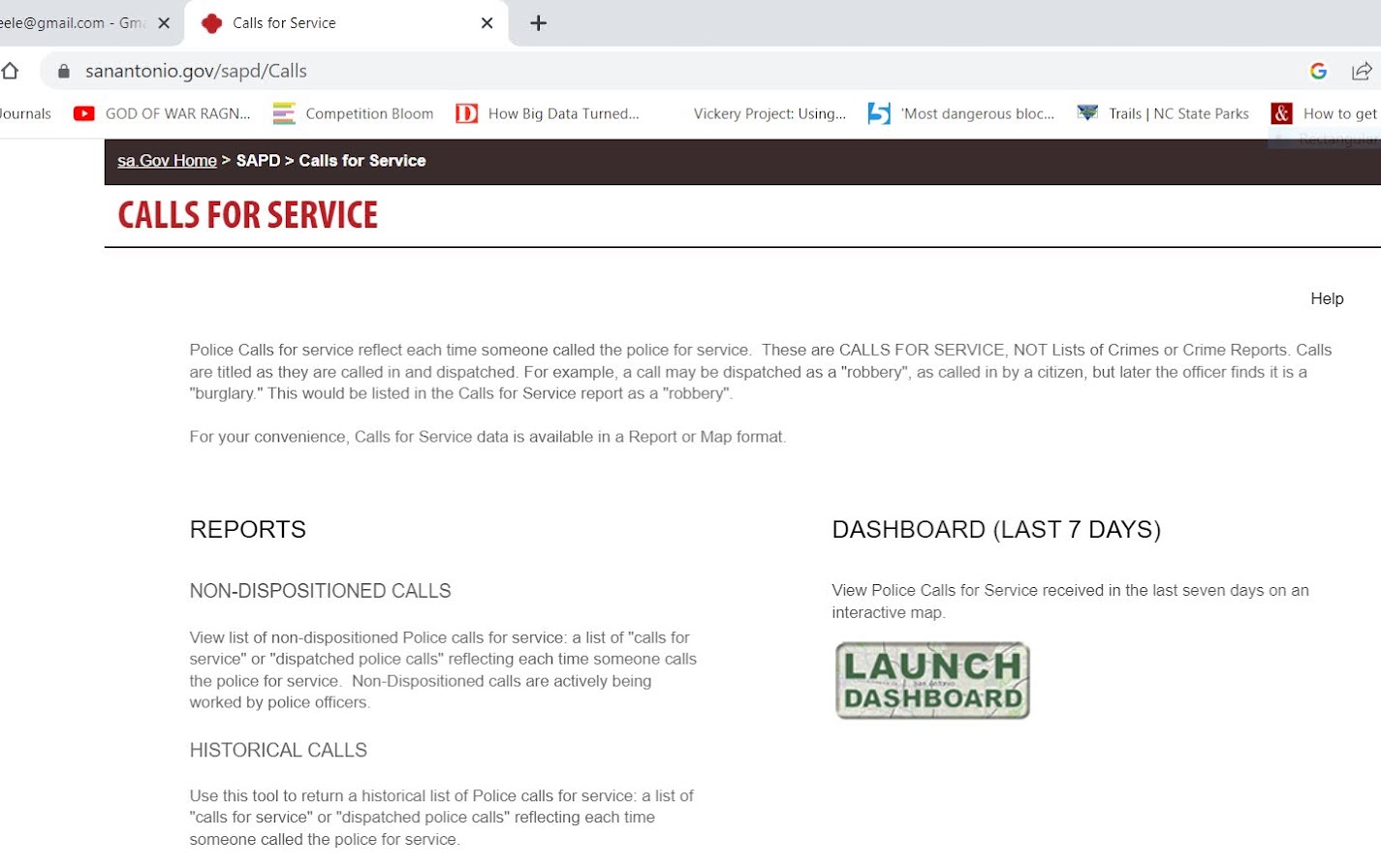
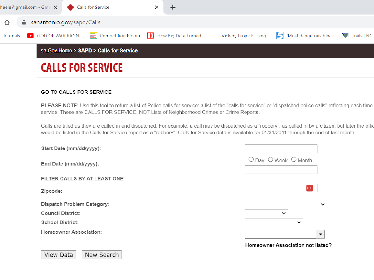
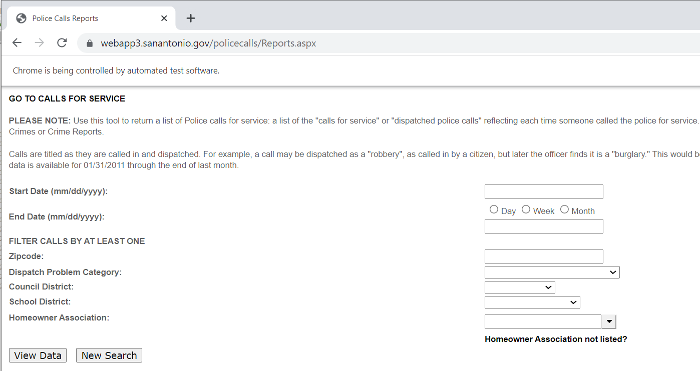
It is tough for me to give general advice about scraping, it involves digging into the source code for a website. Here if you click on the Historical Calls button, the url stays the same, but presents you with a new form page to insert your search parameters:

This is a bit of a red-herring though, it ends up being the entire page is embedded in what is called an i-frame, so the host URL stays the same, but the window inside the webpage changes. On the prior opening page, if you hover over the link for Historical Calls you can see it points to https://webapp3.sanantonio.gov/policecalls/Reports.aspx, so that is page we really need to pay attention to.

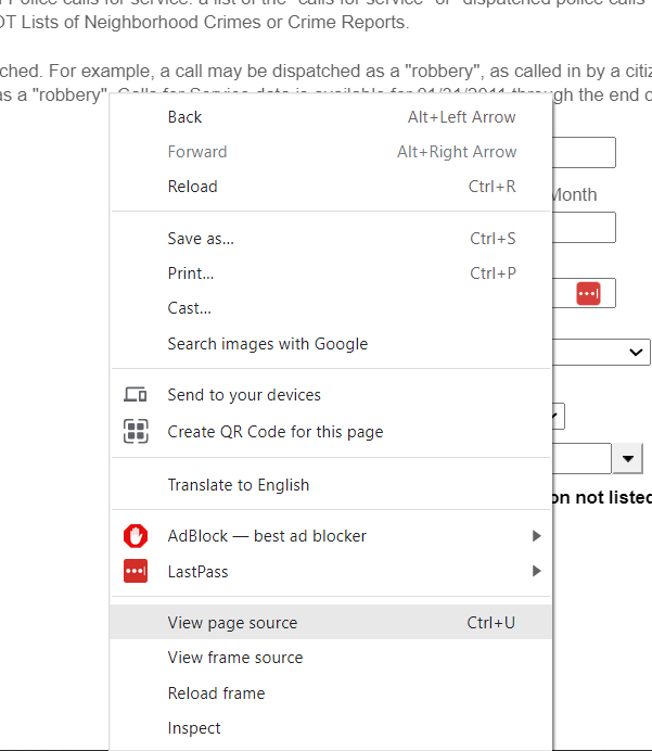
So for general advice, using Chrome to view a web-pages source html, you can right-click and select view-source:

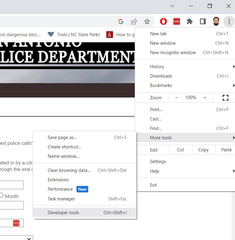
And you can also go into the Developer tools to check out all the items in a page as well.

Typically before worrying about selenium, I study the network tab in here. You want to pay attention to the items that take the longest/have the most data. Typically I am looking for JSON or text files here if I can’t scrape the data directly from the HTML. (Example blog posts grabbing an entire dump of data here, and another finding a hidden/undocumented JSON api using this approach.) Here is an example network call when inputting the search into the San Antonio web-app.

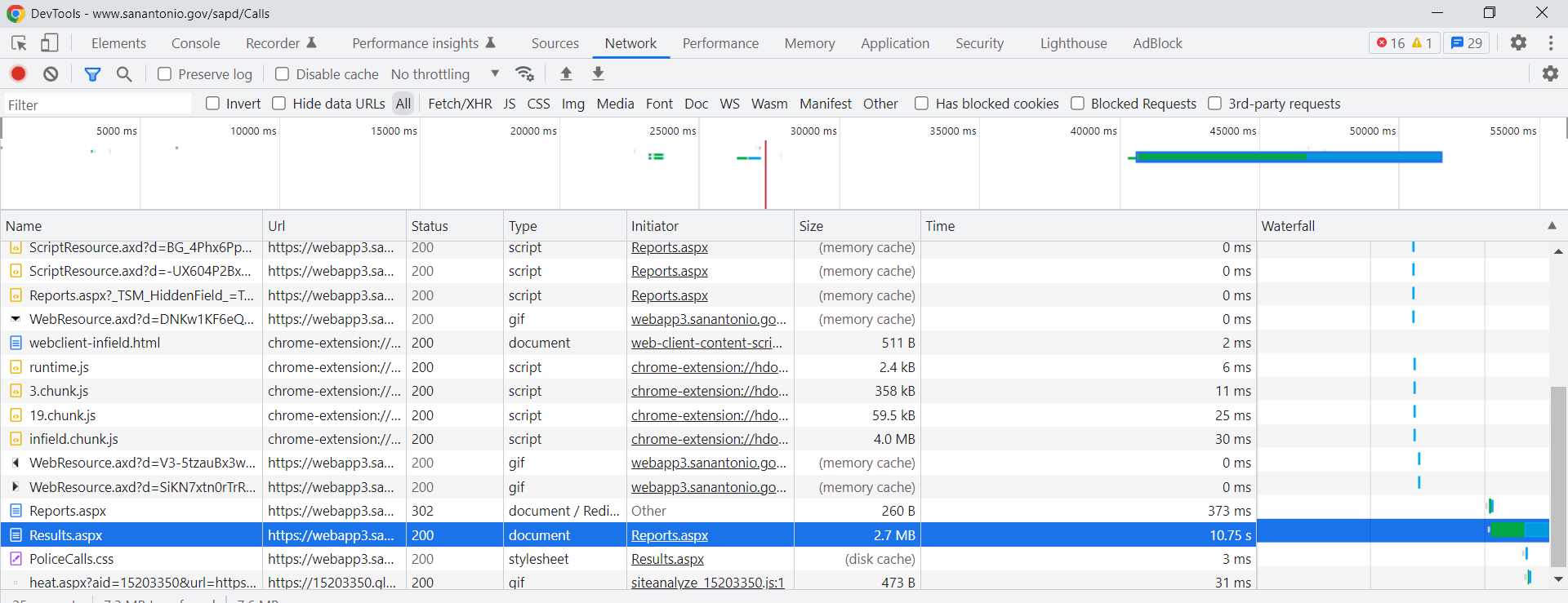
The data is all being transmitted inside of aspx application, not via JSON or other plain text files (don’t take my terminology here as authoritative, I really know near 0% about servers). So we will need to use selenium here. Using python you can install the selenium library, but you also need to download a driver (here I use chrome), and then wherever you save that exe file, add that location to your PATH environment variable.

Now you are ready for the python part.

from selenium import webdriver
from selenium.webdriver.chrome.options import Options
from selenium.webdriver.support.ui import Select
import pandas as pd

# Setting Chrome Options
chrome_options = Options()
#chrome_options.add_argument("-- headless")
chrome_options.add_argument("--window-size=1920,1080")
chrome_options.add_argument("log-level=3")

# Getting the base page
driver = webdriver.Chrome(options=chrome_options)
base_url = "https://webapp3.sanantonio.gov/policecalls/Reports.aspx"
driver = webdriver.Chrome(options=chrome_options)
driver.get(base_url)

Once you run this code, you will see a new browser pop-up. This is great for debugging, but once you get your script finalized, you can see I commented out a line to run in headerless (so it doesn’t bug you by flashing up the browser on your screen).

Now typically what I do is look at the HTML source (like I showed earlier), and then search for the input buttons in HTML. We are trying to figure out the elements we need to insert the data for us to submit a search. Here is the first input for an item we care about, the begin date of the search.

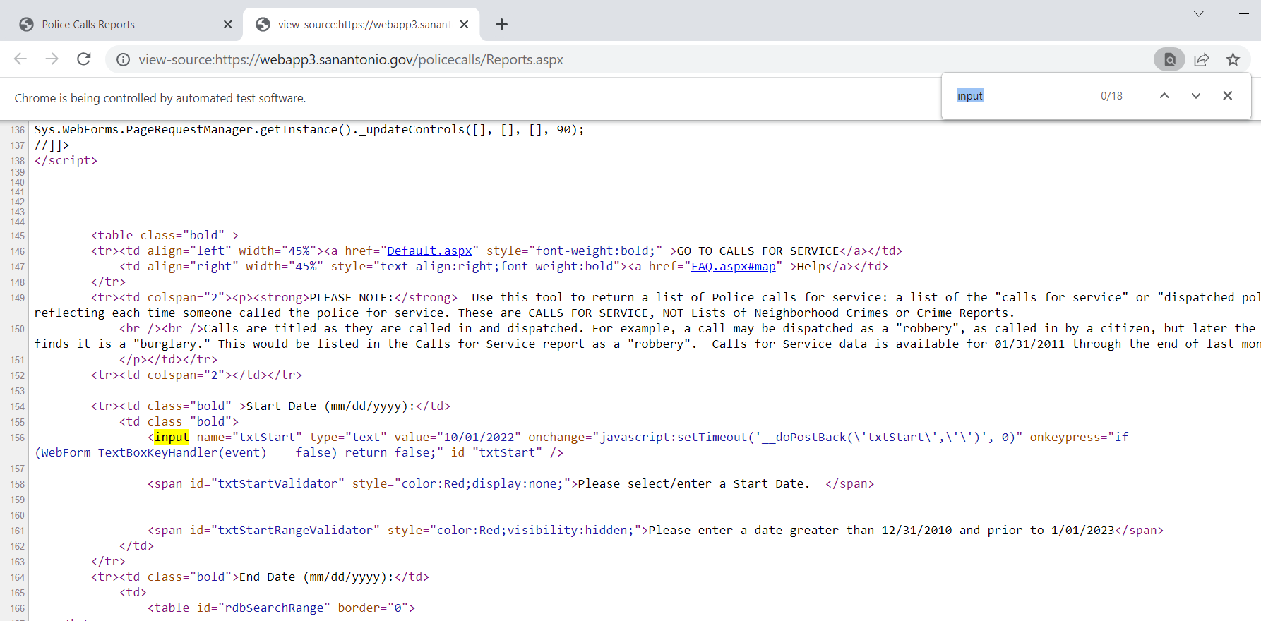
Now we can insert our own date by grabbing the element from the web-page. I grab it here by the “id” attribute in the HTML (many tutorials use xpath, which I am not as familiar with, but at least for these aspx apps what I show works fine). For dates that have a validation stage, you need to not only .send_keys, but to also submit to get past the date validation.

# Inserting date field for begin date
from_date = driver.find_element("id", "txtStart")
from_date.send_keys("10/01/2022")
from_date.submit()

Once you run that code you can actually view the web-page, and see that your date is entered! Now we need to do the same thing for the end date. Then we can put in a plain text zipcode. Since this does not have validation, we do not need to submit it.

# Now for end date
end_date = driver.find_element("id", "txtEndDate")
end_date.send_keys("10/02/2022")
end_date.submit()

# Now inserting text for zipcode
zip = driver.find_element("id", "txtZipcode")
zip.send_keys("78207")
# Sometimes need to clear, zip.clear()

I have a note there on clearing a text box. Sometimes websites have pre-filled options. Sometimes web-sites also do not like .clear(), and you can simulate backspace keystrokes directly. This website does not like it if you clear a date-field for example.

Now the last part, I am going to select a drop-down. If you go into the HTML source again, you can see the list of options.

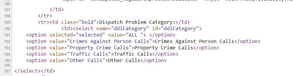
And now we can use the Select function I imported at the beginning to select a particular element of that drop-down. Here I select the crimes against persons.

# Now selecting dropdown
crime_cat = driver.find_element("id", "ddlCategory")
crime_sel = Select(crime_cat)
crime_sel.select_by_visible_text("Crimes Against Person Calls")

Many of these applications have rate limits, so you need to limit the search to tiny windows and subsets, and then loop over the different sets you want to grab all of the data. (Being nice and using time.sleep() between calls to get the results.

Now we are ready to submit the query. The same way you can enter in text into input forms, buttons you can click are also labeled as inputs in the HTML. Here I find the submit button, and then .click() that button. (If there is a direct button to download CSV or some other format, it may make sense to click that button.)

# Now can find the View Data button and submit
view_data = driver.find_element("id", "btnSearch")
view_data.click()

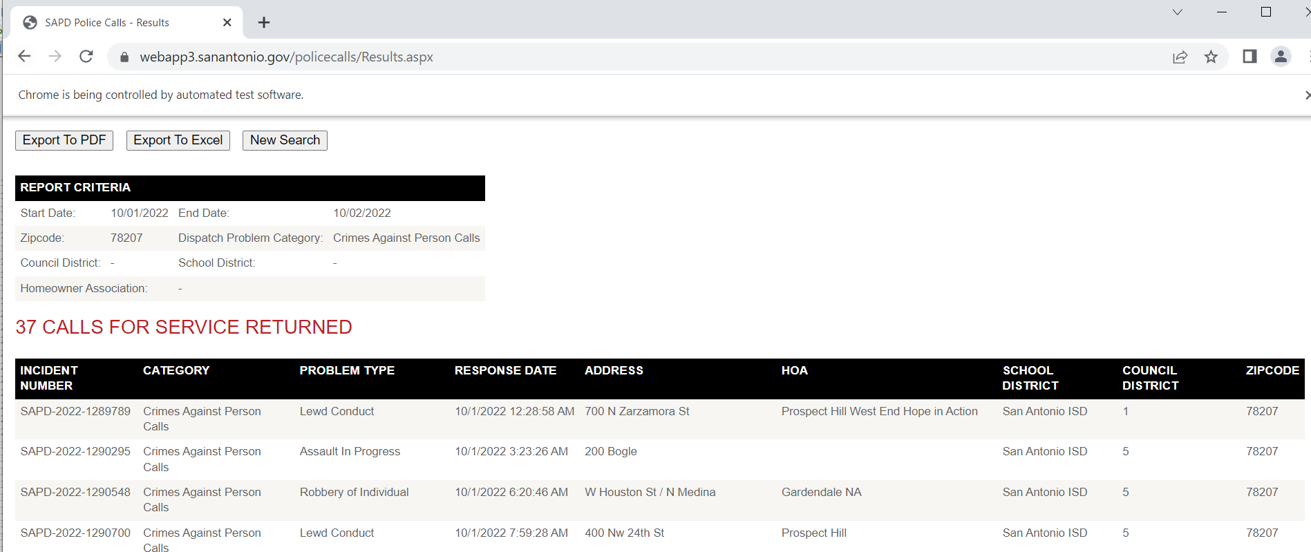
Now that we have our web-page, we can get the HTML source directly and then parse that. Pandas has a nice method to grab tables, and this application is actually very nicely formatted. (I tend to not use this, as many webpages have some very bespoke tables that are hard to grab directly like this). This method grabs all the tables in the web-page by default, here I just want the calls for service table, which has an id of "gvCFS", which I can pass into the pandas .read_html function.

# Pandas has a nice option to read tables directly
html = driver.page_source
cfs = pd.read_html(html, attrs={"id":"gvCFS"})[0]

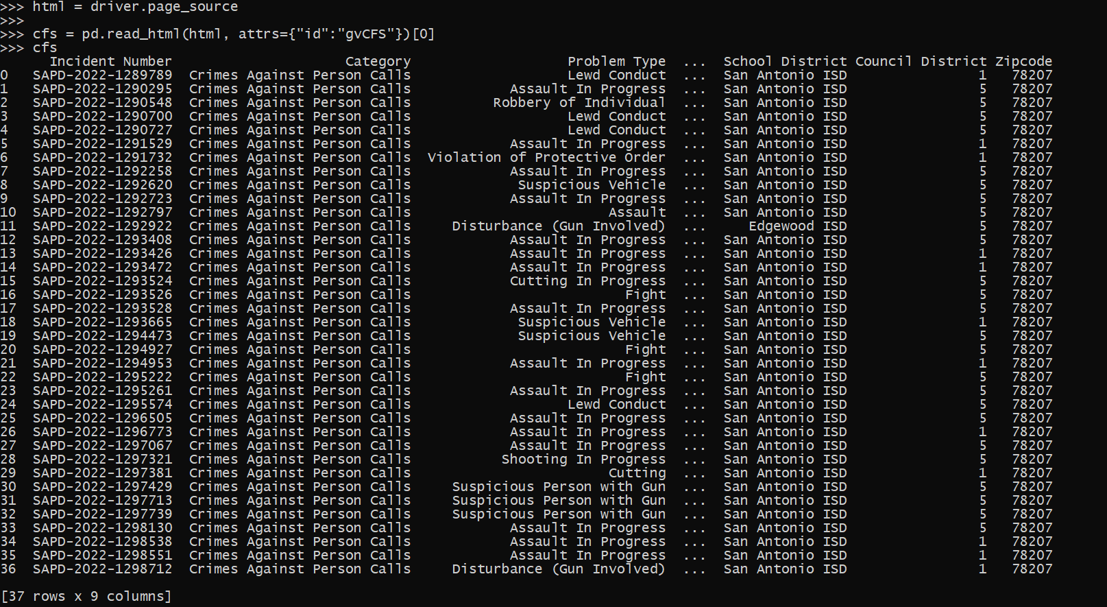
And that shows grabbing a single result. Of course to scrape, you will need to loop over many days (and here different search selections), depending on what data you want to grab. Most of these applications have search limits, so if you do too large a search, will only return the first say 500 results. And San Antonio’s is nice because it returns as a single table in the web-page, most you need to page the results though as well. Which takes further scraping the data and interacting with the page. So it is more painful whenever you need to resort to selenium.

Sometimes pages will point to PDF files, and you can set Chrome’s options to download to a particular location in that scenario (and then use os.rename to name the PDF whatever you want after it is downloaded). You can basically do anything in selenium you can manually, it is often just a tricky set of steps to replicate in code.

Using IO objects in python to read data

Just a quick post on a technique I’ve used a few times recently, in particular when reading web data.

First for a very quick example, in python when reading data with pandas, it often expects a filename on disk. For pandas, e.g. pd.read_csv('my_file.csv'). But if you happen to already have the contents of the csv in a text object in memory, you can use io.StringIO to just read that object.

import pandas as pd
from io import StringIO

# Example csv file inline
examp_csv = """a,b
1,x
2,z"""

pd.read_csv(StringIO(examp_csv))

Where this has come up for me recently is reading in different data from web servers. For example, here is Cary’s API for crime data, you can batch download the whole thing at the below url, but via this approach I currently get an SSL error:

# Town of Cary CSV for crimes
cary_url = 'https://data.townofcary.org/explore/dataset/cpd-incidents/download/?format=csv&timezone=America/New_York&lang=en&use_labels_for_header=true&csv_separator=%2C'

# Returns SSL Error for me
cary_df = pd.read_csv(cary_url)

Note I don’t know the distinction in web server tech that causes this (as sometimes you can just grab a CSV via url, here is an example I have grabbing PPP loan data or with the NIJ recidivism data).

But we can grab the data via requests, and use the same StringIO trick I just showed to get this data:

# Using string IO for reading text
import requests
res_cary = requests.get(cary_url)
cary_df = pd.read_csv(StringIO(res_cary.text))
cary_df

Again I don’t know why some servers you need to go through this approach, but this works for me for Socrata and CartoDB api’s for different cities open data. I also used in recently for converting geojson in ESRI’s api.

The second example I want to show is downloading zipfiles. For this, we will use io.BytesIO instead of StringIO. The census stores various data in zipfiles on their FTP server:

# Example 2, grabbing zipped contents
import zipfile
from io import BytesIO

census_url = 'https://www2.census.gov/programs-surveys/acs/summary_file/2019/data/2019_5yr_Summary_FileTemplates.zip'
req = requests.get(census_url)

# Can use BytesIO for this content
zf = zipfile.ZipFile(BytesIO(req.content))

The zipfile library would be equivalent to reading/extracting a zipfile already on disk. But when downloading there is no need to save to disk, then deal with that file. BytesIO here cuts out the middleman.

Then we gan either grab a specific file inside of our zf object, or extract all the contents one-by-one:

# Now can loop through the list
# or grab specific file
zf.filelist[0]
temp_geo = pd.read_excel(zf.open('2019_SFGeoFileTemplate.xlsx'))
temp_geo.T

Checking for Stale RSS feeds in Python

So while I like RSS feeds, one issue I have noted over the years is that people/companies change the url for the feed. This ends up being a silent error in most feed readers (I swear the google reader had some metrics for this, but that was so long ago).

I have attempted to write code to check for not working feeds at least a few different times and given up. RSS feeds are quite heterogeneous if you look closely. Aliquote had his list though that I started going through to update my own, and figured it would be worth a shot to again filter out old/dormant feeds when checking out new blogs.

So first we will get the blog feeds and Christophe’s tags for each blog:

from bs4 import BeautifulSoup
from urllib.request import Request, urlopen
import pandas as pd
import ssl
import warnings # get warnings for html parser
warnings.filterwarnings("ignore", category=UserWarning, module='bs4')

# aliquotes feed list
feeds = r'https://aliquote.org/pub/urls~'
gcont = ssl.SSLContext()
head = {'User-Agent': 'Chrome/104.0.0.0'}
response = urlopen(Request(feeds,headers=head),context=gcont).read()
list_feeds = response.splitlines()

I do not really know anything about SSL and headers (have had some small nightmares recently on work machines with ZScaler and getting windows subsystem for linux working with poetry/pip). So caveat emptor.

Next we have this ugly function I wrote. It could be cleaned up no doubt, but RSS feeds can fail (either website down, or the url is old/bad), so wrap everything in a try. Also most feeds have items/pubdate tags, but we have a few that have different structure. So all the if/elses are just to capture some of these other formats as best I can.

# Ugly Function to grab RSS last update
def getrss_stats(feed,context=gcont,header=head):
    try:
        req = Request(feed,headers=header)
        response = urlopen(req,context=context)
        soup = BeautifulSoup(response,'html.parser')
        all_items = soup.find_all("item")
        all_pub = soup.find_all("published")
        all_upd = soup.find_all("updated")
        if len(all_items) > 0:
            totn = len(all_items)
            if all_items[0].pubdate:
                last_dt = all_items[0].pubdate.text
            elif all_items[0].find("dc:date"):
                last_dt = all_items[0].find("dc:date").text
            else:
                last_dt = '1/1/1900'
        elif len(all_pub) > 0:
            totn = len(all_pub)
            last_dt = all_pub[0].text
        elif len(all_upd) > 0:
            totn = len(all_upd)
            last_dt = all_upd[0].text
        else:
            totn = 0 # means able to get response
            last_dt = '1/1/1900'
        return [feed,totn,last_dt]
    except:
        return [feed,None,None]

This returns a list of the feed url you put in, as well as the total number of posts in the feed, and the (hopefully) most recent date of a posting. Total numbers is partially a red herring, people may only publish to the feed some limited number of recent blog posts. I fill in missing data from a parsed feed as 0 and ‘1/1/1900’. If the response just overall was bad you get back None values.

So now I can loop over the list of our feeds. Here I only care about those with stats/python/sql (not worrying about Julia yet!):

# Looping over the list
# only care about certain tags
tg = set(['stats','rstats','python','sql'])
fin_stats = []

# Takes a few minutes
for fd in list_feeds:
    fdec = fd.decode().split(" ")
    rss, tags = fdec[0], fdec[1:]
    if (tg & set(tags)):
        rss_stats = getrss_stats(rss)
        rss_stats.append(tags)
        fin_stats.append(rss_stats.copy())

These dates are a bit of a mess. But this is the quickest way to clean them up I know of via some pandas magic:

# Convert data to dataframe
rss_dat = pd.DataFrame(fin_stats,columns=['RSS','TotItems','LastDate','Tags'])

# Coercing everything to a nicer formatted day
rss_dat['LastDate'] = pd.to_datetime(rss_dat['LastDate'].fillna('1/1/1900'),errors='coerce',utc=False)
rss_dat['LastDate'] = pd.to_datetime(rss_dat['LastDate'].astype(str).str[:11])

rss_dat.sort_values(by='LastDate',ascending=False,inplace=True,ignore_index=True)
print(rss_dat.head(10))

And you can see (that links to csv file) that most of Christophe’s feed is up to date. But some are dormant (Peter Norvig’s blog RSS is dormant, but his github he posts snippets/updates), and some have moved to different locations (such as Frank Harrell’s).

So for a feed reader to do something like give a note when a feed has not been updated for say 3 months I think would work for many feeds. Some people have blogs that are not as regular (which is fine), but many sites, such as journal papers, something is probably wrong if no updates for several months.

Use circles instead of choropleth for MSAs

We are homeschooling the kiddo at the moment (the plunge was reading by Bryan Caplan’s approach, and seeing with online schooling just how poor middle school education was). Wife is going through AP biology at the moment, and we looked up various job info on biomedical careers. Subsequently came across this gem of a map of MSA estimates from the Bureau of Labor Stats (BLS) Occupational Employment and Wage Stats series (OES).

I was actually mapping some metro stat areas (MSAs) at work the other day, and these are just terrifically bad geo areas to show via a choropleth map. All choropleth maps have the issue of varying size areas, but I never realized having somewhat regular borders (more straight lines) makes the state and county maps not so bad – these MSA areas though are tough to look at. (Wife says it scintillates for her if she looks too closely.)

There are various incredibly tiny MSAs next to giant ones that you will just never see in these maps (no matter what color scheme you use). Nevada confused for me quite a bit, until I zoomed in to see that there are 4 areas, Reno is just a tiny squib.

Another example is Boulder above Denver. (Look closely at the BLS map I linked, you can just make out Boulder if you squint, but I cannot tell what color it corresponds to in the legend.) The outline heavy OES maps, which are mostly missing data, are just hopeless to display like this effectively. Reno could be the hottest market for whatever job, and it will always be lost in this map if you show employment via the choropleth approach. So of course I spent the weekend hacking together some maps in python and folium.

The BLS has a public API, but I was not able to find the OES stats in that. But if you go through the motions of querying the data and muck around in the source code for those queries, you can see they have an undocumented API call to generate json to fill the tables. Then using this tool to convert the json calls to python (thank you Hacker News), I was able to get those tables into python.

I have these functions saved on github, so check out that source for the nitty gritty. But just here quickly, here is a replicated choropleth map, showing the total employees for bio jobs (you can go to here to look up the codes, or run my function bls_maps.ocodes() to get a pandas dataframe of those fields).

# Creating example bls maps
from bls_geo import *

# can check out https://www.bls.gov/oes/current/oes_stru.htm
bio = '172031'
bio_stats = oes_geo(bio)
areas = get_areas() # this takes a few minutes
state = state_albers()
geo_bio = merge_occgeo(bio_stats,areas)

ax = geo_bio.plot(column='Employment',cmap='inferno',legend=True,zorder=2)
state.boundary.plot(ax=ax,color='grey',linewidth=0.5,zorder=1)
ax.set_ylim(0.1*1e6,3.3*1e6)
ax.set_xlim(-0.3*1e7,0.3*1e7)   # lower 48 focus (for Albers proj)
ax.set_axis_off()
plt.show()

And that is not much better than BLSs version. For this data, if you are just interested in looking up or seeing the top metro areas, just doing a table, e.g. above geo_bio.to_excel('biojobs.xlsx'), works just as well as a map.

So I was surprised to see Minneapolis pop up at the top of that list (and also surprised Raleigh doesn’t make the list at all, but Durham has a few jobs). But if you insist on seeing spatial trends, I prefer to go the approach of mapping proportion or graduate circles, placing the points at the centroid of the MSA:

att = ['areaName','Employment','Location Quotient','Employment per 1,000 jobs','Annual mean wage']
form = ['',',.0f','.2f','.2f',',.0f']

map_bio = fol_map(geo_bio,'Employment',['lat', 'lon'],att,form)
#map_bio.save('biomap.html')
map_bio #if in jupyter can render like this

I am too lazy to make a legend, you can check out nbviewer to see an interactive Folium map, which I have tool tips (similar to the hover for the BLS maps).

Forgive my CSS/HTML skills, not sure how to make nicer popups. So you lose the exact areas these MSA cover in this approach, but I really only expect a general sense from these maps anyway.

These functions are general enough for whatever wage series you want (although these functions will likely break when the 2021 data comes out). So here is the OES table for data science jobs:

I feel going for the 90th percentile (mapping that to the 10 times programmer) is a bit too over the top. But I can see myself reasonably justifying 75th percentile. (Unfortunately these agg tables don’t have a way to adjust for years of experience, if you know of a BLS micro product I could do that with let me know!). So you can see here the somewhat inflated salaries for the SanFran Bay area, but not as inflated as many might have you think (and to be clear, these are for 2020 survey estimates).

If we look at map of data science jobs, varying the circles by that 75th annual wage percentile, it looks quite uniform. What happens is we have some real low outliers (wages under 70k), resulting in tiny circles (such as Athen’s GA). Most of the other metro regions though are well over 100k.

In more somber news, those interactive maps are built using Leaflet as the backend, which was create by a Ukranian citizen, Vladimir Agafonkin. We can do amazing things with open source code, but we should always remember it is on the backs of someones labor we are able to do those things.

Downloading your PDFs from CiteULike using python and selenium

CiteULike, an online bibliography manager, is unfortunately shutting down. They have a service to export your bibliography as a BibTex file, but this does not include the PDFs you have uploaded to the site. Having web access to the PDFs is one of the main reasons I liked CiteULike (along with the tag cloud).

I have too many PDFs to download them all manually (over 2,000), so I wrote a script in Python to download the PDFs. Unlike prior scraping examples I’ve written about, you need to have signed into your CiteULike account to be able to download the files. Hence I use the selenium library to mimic what you do normally in a web-browser.

So let me know what bibliography manager I should switch to. Really one of the main factors will be if I can automate the conversion, including PDFs (even if it just means pointing to where the PDF is stored on my local machine).

This is a good tutorial to know about even if you don’t have anything to do with CiteULike. There are various web services that you need to sign in or mimic the browser like this to download data repeatedly, such as if a PD has a system where you need to input a set of dates to get back crime incidents (and limit the number returned, so you need to do it repeatedly to get a full sample). The selenium library can be used in a similar fashion to this tutorial in that circumstance.

Scraping Meth Labs with Python

For awhile in my GIS courses I have pointed to the DEA’s website that has a list of busted meth labs across the county, named the National Clandestine Laboratory Register. Finally a student has shown some interest in this, and so I spent alittle time writing a scraper in Python to grab the data. For those who would just like the data, here I have a csv file of the scraped labs that are geocoded to the city level. And here is the entire SPSS and Python script to go from the original PDF data to the finished product.

So first off, if you visit the DEA website, you will see that each state has its own PDF file (for example here is Texas) that lists all of the registered labs, with the county, city, street address, and date. To turn this into usable data, I am going to do three steps in Python:

  1. download the PDF file to my local machine using urllib python library
  2. convert that PDF to an xml file using the pdftohtml command line utility
  3. use Beautifulsoup to parse the xml file

I will illustrate each in turn and then provide the entire Python script at the end of the post.

So first, lets import the libraries we need, and also note I downloaded the pdftohtml utility and placed that location as a system path on my Windows machine. Then we need to set a folder where we will download the files to on our local machine. Finally I create the base url for our meth labs.

from bs4 import BeautifulSoup
import urllib, os

myfolder = r'C:\Users\axw161530\Dropbox\Documents\BLOG\Scrape_Methlabs\PDFs' #local folder to download stuff
base_url = r'https://www.dea.gov/clan-lab' #online site with PDFs for meth lab seizures

Now to just download the Texas pdf file to our local machine we would simply do:

a = 'tx'
url = base_url + r'/' + a + '.pdf'
file_loc = os.path.join(myfolder,a)
urllib.urlretrieve(url,file_loc + '.pdf')

If you are following along and replaced the path in myfolder with a folder on your personal machine, you should now see the Texas PDF downloaded in that folder. Now I am going to use the command line to turn this PDF into an xml document using the os.system() function.

#Turn to xml with pdftohtml, does not need xml on end
cmd = 'pdftohtml -xml ' + file_loc + ".pdf " + file_loc
os.system(cmd)

You should now see that there is an xml document to go along with the Texas file. You can check out its format using a text editor (wordpress does not seem to like me showing it here).

So basically we can use the top and the left attributes within the xml to identify what row and what column the items are in. But first, we need to read in this xml and turn it into a BeautifulSoup object.

MyFeed = open(file_loc + '.xml')
textFeed = MyFeed.read()
FeedParse = BeautifulSoup(textFeed,'xml')
MyFeed.close()

Now the FeedParse item is a BeautifulSoup object that you can query. In a nutshell, we have a top level page tag, and then within that you have a bunch of text tags. Here is the function I wrote to extract that data and dump it into tuples.

#Function to parse the xml and return the line by line data I want
def ParseXML(soup_xml,state):
    data_parse = []
    page_count = 1
    pgs = soup_xml.find_all('page')
    for i in pgs:
        txt = i.find_all('text')
        order = 1
        for j in txt:
            value = j.get_text() #text
            top = j['top']
            left = j['left']
            dat_tup = (state,page_count,order,top,left,value)
            data_parse.append(dat_tup)
            order += 1
        page_count += 1
    return data_parse

So with our Texas data, we could call ParseXML(soup_xml=FeedParse,state=a) and it will return all of the data nested in those text tags. We can just put these all together and loop over all of the states to get all of the data. Since the PDFs are not that large it works quite fast, under 3 minutes on my last run.

from bs4 import BeautifulSoup
import urllib, os

myfolder = r'C:\Users\axw161530\Dropbox\Documents\BLOG\Scrape_Methlabs\PDFs' #local folder to download stuff
base_url = r'https://www.dea.gov/clan-lab' #online site with PDFs for meth lab seizures
                                           #see https://www.dea.gov/clan-lab/clan-lab.shtml
state_ab = ['al','ak','az','ar','ca','co','ct','de','fl','ga','guam','hi','id','il','in','ia','ks',
            'ky','la','me','md','ma','mi','mn','ms','mo','mt','ne','nv','nh','nj','nm','ny','nc','nd',
            'oh','ok','or','pa','ri','sc','sd','tn','tx','ut','vt','va','wa','wv','wi','wy','wdc']
            
state_name = ['Alabama','Alaska','Arizona','Arkansas','California','Colorado','Connecticut','Delaware','Florida','Georgia','Guam','Hawaii','Idaho','Illinois','Indiana','Iowa','Kansas',
              'Kentucky','Louisiana','Maine','Maryland','Massachusetts','Michigan','Minnesota','Mississippi','Missouri','Montana','Nebraska','Nevada','New Hampshire','New Jersey',
              'New Mexico','New York','North Carolina','North Dakota','Ohio','Oklahoma','Oregon','Pennsylvania','Rhode Island','South Carolina','South Dakota','Tennessee','Texas',
              'Utah','Vermont','Virginia','Washington','West Virginia','Wisconsin','Wyoming','Washington DC']

all_data = [] #this is the list that the tuple data will be stashed in

#Function to parse the xml and return the line by line data I want
def ParseXML(soup_xml,state):
    data_parse = []
    page_count = 1
    pgs = soup_xml.find_all('page')
    for i in pgs:
        txt = i.find_all('text')
        order = 1
        for j in txt:
            value = j.get_text() #text
            top = j['top']
            left = j['left']
            dat_tup = (state,page_count,order,top,left,value)
            data_parse.append(dat_tup)
            order += 1
        page_count += 1
    return data_parse

#This loops over the pdfs, downloads them, turns them to xml via pdftohtml command line tool
#Then extracts the data

for a,b in zip(state_ab,state_name):
    #Download pdf
    url = base_url + r'/' + a + '.pdf'
    file_loc = os.path.join(myfolder,a)
    urllib.urlretrieve(url,file_loc + '.pdf')
    #Turn to xml with pdftohtml, does not need xml on end
    cmd = 'pdftohtml -xml ' + file_loc + ".pdf " + file_loc
    os.system(cmd)
    #parse with BeautifulSoup
    MyFeed = open(file_loc + '.xml')
    textFeed = MyFeed.read()
    FeedParse = BeautifulSoup(textFeed,'xml')
    MyFeed.close()
    #Extract the data elements
    state_data = ParseXML(soup_xml=FeedParse,state=b)
    all_data = all_data + state_data

Now to go from those sets of tuples to actually formatted data takes a bit of more work, and I used SPSS for that. See here for the full set of scripts used to download, parse and clean up the data. Basically it is alittle more complicated than just going from long to wide using the top marker for the data as some rows are off slightly. Also there is complications for long addresses being split across two lines. And finally there are just some data errors and fields being merged together. So that SPSS code solves a bunch of that. Also that includes scripts to geocode the to the city level using the Google geocoding API.

Let me know if you do any analysis of this data! I quickly made a time series map of these events via CartoDB. You can definately see some interesting patterns of DEA concentration over time, although I can’t say if that is due to them focusing on particular areas or if they are really the areas with the most prevalent Meth lab problems.

Some GIS data scraping adventures: Banksy graffiti and gang locations in NYC

I’ve recently scraped some geographic data that I may use in my graduate level GIS course. I figured I would share with everyone, and take some time to describe for others how I scraped the data.

So to start, if you read an online article and it has a webmap with some GIS data in it – the data exists somewhere. It won’t always be the case that you can actually download the data, but for the most current and popular interactive mapping tools, the data is often available if you know where to look.

For example, I asked on the GIS stackexchange site awhile ago how can you download the point data in this NYC homicide map from the Times. I had emailed the reporters multiple times and they did not respond. A simple solution the answerers suggested was to use website developer tools to see what was being loaded when I refreshed the page. It happened that the map is being populated by a two simple text files (1,2).

It may be an interesting project to see how this compares (compiling via news stories) versus official data, which NYC recently released going back to 2006. Especially since such crowdsourced news datasets are used for other things, like counting mass shootings.

The two example mapping datasets I provide below though are a bit different process to get the underlying data – but just as easy. Many current webmaps use geojson files as the backend. What I did for the two examples below is I just looked at the html source for the website, and look for json data formats – links that specify “js” or “json” extensions. If you click through those external json links you can see if they have the data.

The other popular map type though comes from ESRI. You can typically find an ESRI server populating the map, and if the website has say a parcel data lookup you can often find an ESRI geocoding server (see here for one example of using an ESRI geocoding api). The maps though unfortunately do not always have exposed data. Sometimes what looks like vector data are actually just static PNG tiles. Council Districts in this Dallas map are an example. If you dig deep enough, you can find the PNG tiles for the council districts, but that does not do anyone much good. Pretty much all of those layers are available for download from other sources though. A similar thing happens with websites with crime reports, such as RAIDS Online or CrimeReports.com. They intentionally build the web map so you cannot scrape the data.

So that said, before we go further though – it should go without saying that you should not steal/plagiarize people’s articles or simply rip-off their graphics. Conducting new analysis with the publicly available data though seems fair game to me.

Banksy Taggings in NYC

There was a recent stink in the press about Kim Rossmo and company using geographic offender profiling to identify the likely home location of the popular graffiti artist Banksy. Here is the current citation of the journal article for those interested:

Hauge, M. V., Stevenson, M. D., Rossmo, D. K., and Le Comber, S. C. (2016). Tagging banksy: using geographic profiling to investigate a modern art mystery. Journal of Spatial Science, pages 1-6. doi:10.1080/14498596.2016.1138246

The article uses data from Britain, so I looked up to see if his taggings in other places was available. I came across this article showing a map of locations in New York City. So I searched where the data was coming from, and found the json file that contains the point data here. I just built a quick excel spreadsheet to parse the data, and you can download that spreadsheet here.

Gang Locations

This article posts a set of gang territories in NYC. This is pretty unique – I am unfamiliar with any other public data source that identifies gang territories. So I figured it would be a potential fun project for students in my GIS course – for instance in overlaying with the 311 graffiti data.

Again the data at the backend is in json format, and can be found here. To convert this data to a shapefile is a bit challenging, as it has points, lines and polygons all in the same file. What I did was buffer the lines and points by a small amount to be able to stuff them all in one shapefile. A zip file of that shapefile can be downloaded here.

Drop me a note if you use this data, I’d be interested in your analyses! Hence why I am sharing the data for others to play with 🙂

A shout out for ScraperWiki

I’ve used the online tool ScraperWiki a few times to scrape some online data into a simple spreadsheet. It provides a set of tools to code in Python (and a few other languages) online in the browser and dump the resulting set of information into an online table. It also allows you to set the data collection on a timer and updates the table with new information. It is just a nice set of tools that makes getting and sharing the data easier.

For a few sample scripts I’ve used it for in the past:

  • Grabbing the number of chat posts from Stack Overflow chat rooms.
  • Grabbing the user location from profiles on the GIS.SE site. (This is really redundant with the power to query the SO data explorer – it can be more up to date though.)
  • Scraping the NYPD reported precinct statistics that were uploaded in PDF form. (Yes you can turn PDFs into xml which you can subsequently parse).

I previously used what is now called ScraperWiki Classic. But since the service is migrating to a new platform my prior scripts will not continue downloading data.

It appears my NYPD data scraper does not work any more anyway (they do have an online map now – but unfortunately are not providing the data in a convenient format for bulk download to the NYC Open Data site last I knew). But it has some historical data from the weekly precinct level crime stats between the end of 2010 and through most of 2013 if you are interested.

I’ve migrated the chat posts scraper to the new site, and so it will continue to update with new data for the activity in the SO R Room and the main chat room on the CrossValidated Stats Site. I’ll have to leave analysing that data for a future post, but if you are interested in amending the scraper to download data for a different room it is pretty easy. Just fork it and add/change the rooms of interest to the url_base array. You can download a csv file of the data directly from this link. The Mono field is a count of the unique "Monologue" tags in the html, and the Baseroom shows what chat room the data is from. Note that the Mono value shows 0 even if the room did not exist at that date.

I’m not sure how to make the scraper viewable to the public, but you can still view the code on the classic site. Note the comment about the CPU time isn’t applicable to the main site; I could download the transcripts all the way back to 2010 and I did not receive any errors from ScraperWiki.