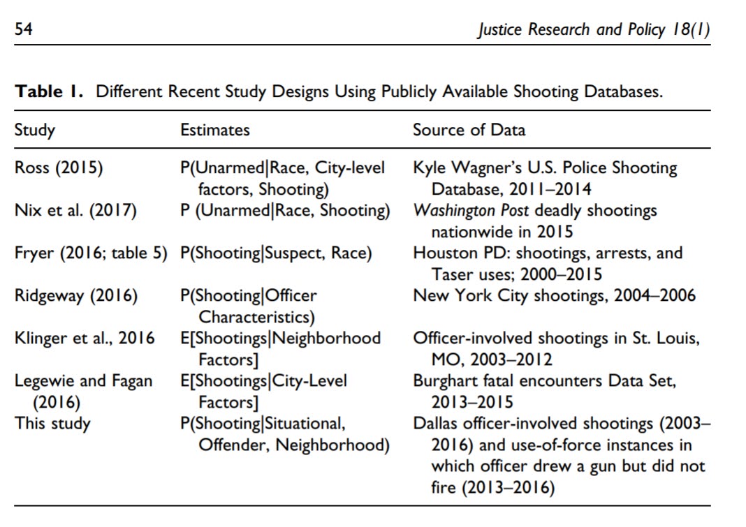
Marisa Iati interviewed me for a few clips in a recent update of the WaPo data on officer involved fatal police shootings. I’ve written in the past the data are very consistent with a Poisson process, and this continues to be true.

So first thing Marisa said was that shootings in 2021 are at 1055 (up from 1021 in 2020). Is this a significant increase? I said no off the cuff – I knew the average over the time period WaPo has been collecting data is around 1000 fatal shootings per year, so given a Poisson distribution mean=variance, we know the standard deviation of the series is close to sqrt(1000), which approximately equals 60. So anything 1000 plus/minus 60 (i.e. 940-1060) is within the typical range you would expect.

In every interview I do, I struggle to describe frequentist concepts to journalists (and this is no different). This is not a critique of Marisa, this paragraph is certainly not how I would write it down on paper, but likely was the jumble that came out of my mouth when I talked to her over the phone:

Despite setting a record, experts said the 2021 total was within expected bounds. Police have fatally shot roughly 1,000 people in each of the past seven years, ranging from 958 in 2016 to last year’s high. Mathematicians say this stability may be explained by Poisson’s random variable, a principle of probability theory that holds that the number of independent, uncommon events in a large population will remain fairly stagnant absent major societal changes.

So this sort of mixes up two concepts. One, the distribution of fatal officer shootings (a random variable) can be very well approximated via a Poisson process. Which I will show below still holds true with the newest data. Second, what does this say about potential hypotheses we have about things that we think might influence police behavior? I will come back to this at the end of the post,

R Analysis at the Daily Level

So my current ptools R package can do a simple analysis to show that this data is very consistent with a Poisson process. First, install the most recent version of the package via devtools, then you can read in the WaPo data directly via the Github URL:

library(devtools)
install_github("apwheele/ptools")
library(ptools)

url <- 'https://raw.githubusercontent.com/washingtonpost/data-police-shootings/master/fatal-police-shootings-data.csv'
oid <- read.csv(url,stringsAsFactors = F)

Looking at the yearly statistics (clipping off events recorded so far in 2022), you can see that they are hypothetically very close to a Poisson distribution with a mean/variance of 1000, although perhaps have a slow upward trend over the years.

# Year Stats
oid$year <- as.integer(substr(oid$date,1,4))
year_stats <- table(oid$year)
print(year_stats)
mean(year_stats[1:7]) # average of 1000 per year
var(year_stats[1:7])  # variance just under 1000

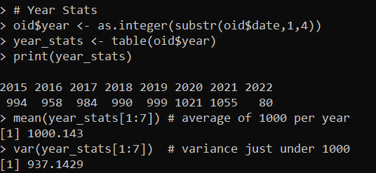
We can also look at the distribution at shorter time intervals, here per day. First I aggregat the data to the daily level (including 0 days), second I use my check_pois function to get the comparison distributions:

#Now aggregating to count per day
oid$date_val <- as.Date(oid$date)
date_range <- paste0(seq(as.Date('2015-01-01'),max(oid$date_val),by='days'))
day_counts <- as.data.frame(table(factor(oid$date,levels=date_range)))
head(day_counts)

pfit <- check_pois(day_counts$Freq, 0, 10, mean(day_counts$Freq))
print(pfit)

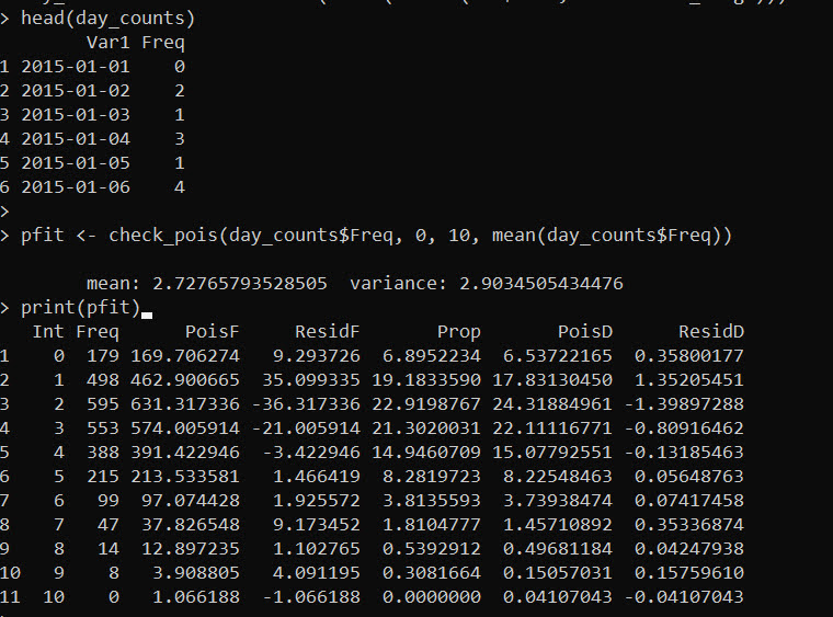
The way to read this, for a mean of 2.7 fatal OIS per day (and given this many days), we would expect 169.7 0 fatality days in the sample (PoisF), but we actually observed 179 0 fatality days, so a residual of 9.3 in the total count. The trailing rows show the same in percentage terms, so we expect 6.5% of the days in the sample to have 0 fatalities according to the Poisson distribution, and in the actual data we have 6.9%.

You can read the same for the rest of the rows, but it is mostly the same. It is only very slight deviations from the baseline Poisson expected Poisson distribution. This data is the closest I have ever seen to real life, social behavioral data to follow a Poisson process.

For comparison, lets compare to the NYC shootings data I have saved in the ptools package.

# Lets check against NYC Shootings
data(nyc_shoot)
date_range <- paste0(seq(as.Date('2006-01-01'),max(nyc_shoot$OCCUR_DATE),by='days'))
shoot_counts <- as.data.frame(table(factor(nyc_shoot$OCCUR_DATE,levels=date_range)))

sfit <- check_pois(shoot_counts$Freq,0,max(shoot_counts$Freq),mean(shoot_counts$Freq))
round(sfit,1)

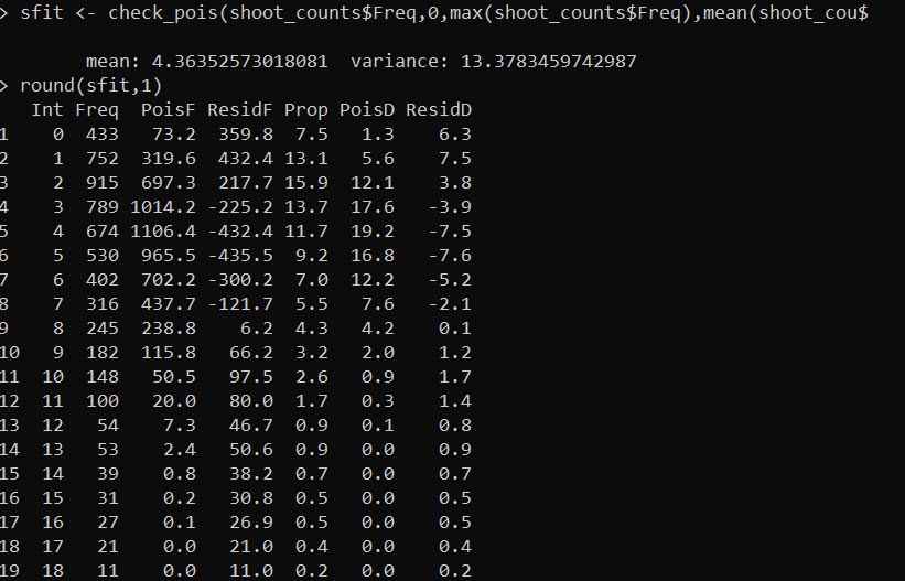
This is much more typical of crime data I have analyzed over my career (in that it deviates from a Poisson process by quite a bit). The mean is 4.4 shootings per day, but the variance is over 13. There are many more 0 days than expected (433 observed vs 73 expected). And there are many more high crime shooting days than expected (tail of the distribution even cut off). For example there are 27 days with 18 shootings, whereas a Poisson process would only expect 0.1 days in a sample of this size.

My experience though is that when the data is overdispersed, a negative binomial distribution will fit quite well. (Many people default to a zero-inflated, like Paul Allison I think that is a mistake unless you have a structural reason for the excess zeroes you want to model.)

So here is an example of fitting a negative binomial to the shooting data:

# Lets fit a negative binomial and check out
library(fitdistrplus)
fnb <- fitdist(shoot_counts$Freq,"nbinom")
print(fnb$estimate)

sfit$nb <- 100*mapply(dnbinom, x=sfit$Int, size=fnb$estimate[1], mu=fnb$estimate[2])
round(sfit[,c('Prop','nb')],1) # Much better overall fit

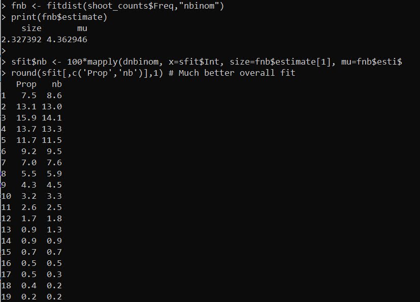
And this compares the percentages. So you can see observed 7.5% 0 shooting days, and expected 8.6% according to this negative binomial distribution. Much closer than before. And the tails are fit much closer as well, for example, days with 18 shootings are expected 0.2% of the time, and are observed 0.4% of the time.

So What Inferences Can We Make?

In social sciences, we are rarely afforded the ability to falsify any particular hypothesis – or in more lay-terms we can’t really ever prove something to be false beyond a reasonable doubt. We can however show whether empirical data is consistent or inconsistent with any particular hypothesis. In terms of Fatal OIS, several ready hypotheses ones may be interested in are Does increased police scrutiny result in fewer OIS?, or Did the recent increase in violence increase OIS?.

While these two processes are certainly plausible, the data collected by WaPo are not consistent with either hypothesis. It is possible both mechanisms are operating at the same time, and so cancel each other out, to result in a very consistent 1000 Fatal OIS per year. A simpler explanation though is that the baseline rate has not changed over time (Occam’s razor).

Again though we are limited in our ability to falsify these particular hypotheses. For example, say there was a very small upward trend, on the order of something like +10 Fatal OIS per year. Given the underlying variance of Poisson variables, even with 7+ years of data it would be very difficult to identify that small of an upward trend. Andrew Gelman likens it to measuring the weight of a feather carried by a Kangaroo jumping on the scale.

So really we could only detect big changes that swing OIS by around 100 events per year I would say offhand. Anything smaller than that is likely very difficult to detect in this data. And so I think it is unlikely any of the recent widespread impacts on policing (BLM, Ferguson, Covid, increased violence rates, whatever) ultimately impacted fatal OIS in any substantive way on that order of magnitude (although they may have had tiny impacts at the margins).

Given that police departments are independent, this suggests the data on fatal OIS are likely independent as well (e.g. one fatal OIS does not cause more fatal OIS, nor the opposite one fatal OIS does not deter more fatal OIS). Because of the independence of police departments, I am not sure there is a real great way to have federal intervention to reduce the number of fatal OIS. I think individual police departments can increase oversight, and maybe state attorney general offices can be in a better place to use data driven approaches to oversee individual departments (like ProPublica did in New Jersey). I wouldn’t bet money though on large deviations from that fatal 1000 OIS anytime soon though.

So besides code on my GitHub page, I have a list of various statistic functions I’ve scripted on the blog over the years on my code snippets page. One of those functions I will illustrate today is some R code to check the fit of the Poisson distribution. Many of my crime analysis examples rely on crime data being approximately Poisson distributed. Additionally it is relevant in regression model building, e.g. should I use a Poisson GLM or do I need to use some type of zero-inflated model?

Here is a brief example to show how my R code works. You can source it directly from my dropbox page. Then I generated 10k simulated rows of Poisson data with a mean of 0.2. So I see many people in CJ make the mistake that, OK my data has 85% zeroes, I need to use some sort of zero-inflated model. If you are working with very small spatial/temporal units of analysis and/or rare crimes, it may be the mean of the distribution is quite low, and so the Poisson distribution is actually quite close.

# My check Poisson function
source('https://dl.dropboxusercontent.com/s/yj7yc07s5fgkirz/CheckPoisson.R?dl=0')

# Example with simulated data
set.seed(10)
lambda <- 0.2
x <- rpois(10000,lambda)
CheckPoisson(x,0,max(x),mean(x))

Here you can see in the generated table from my CheckPoisson function, that with a mean of 0.2, we expect around 81.2% zeroes in the data. And since we simulated the data according to the Poisson distribution, that is what we get. The table shows that out of the 10k simulation rows, 8121 were 0’s, 1692 rows were 1’s etc.

In real life data never exactly conform to hypothetical distributions. But we often want to see how close they are to the hypothetical before building predictive models. A real life example as close to Poisson distributed data as I have ever seen is the Washington Post Fatal Use of Force data. Every year WaPo has been collating the data, the total number of Fatal uses of Police Force in the US have been very close to 1000 events per year. And even in all the turmoil this past year, that is still the case.

# Washington Post Officer Involved Shooting Deaths Data
oid <- read.csv('https://raw.githubusercontent.com/washingtonpost/data-police-shootings/master/fatal-police-shootings-data.csv',
                stringsAsFactors = F)

# Year Stats
oid$year <- as.integer(substr(oid$date,1,4))
year_stats <- table(oid$year)[1:6]
year_stats 
mean(year_stats)
var(year_stats)

One way to check the Poison distribution is that the mean and the variance should be close, and here at the yearly level the data have some evidence of underdispersion according to the Poisson distribution (most crime data is overdispersed – the variance is much greater than the mean). If the actual mean is around 990, you would expect typical variations of say around plus/minus 60 per year (~ 2*sqrt(990)). But that only gives us a few observations to check (6 years). We can dis-aggregate the data to smaller intervals and check the Poisson assumption. Here I aggregate to days (note that this includes zero days in the table levels calculation). Then we again check the fit of the Poisson distribution.

#Now aggregating to count per day
oid$date_val <- as.Date(oid$date)
date_range <- paste0(seq(as.Date('2015-01-01'),max(oid$date_val),by='days'))
day_counts <- as.data.frame(table(factor(oid$date,levels=date_range)))
head(day_counts)
pfit <- CheckPoisson(day_counts$Freq, 0, 10, mean(day_counts$Freq))
pfit

According to the mean and the variance, it appears the distribution is a very close fit to the Poisson. We can see in this data we expected to have around 147 days with 0 fatal encounters, and in reality there were 160. I like seeing the overall counts, but another way is via the proportions in the final three columns of the table. You can see for all of the integers, we are less than 2 percentage points off for any particular integer count. E.g. we expect the distribution to have 3 fatal uses of force on about 22% of the days, but in the observed distribution days with 3 events only happened around 21% of the days (or 20.6378132 without rounding). So overall these fatal use of force data of course are not exactly Poisson distributed, but they are quite close.

So the Poisson distribution is motivated via a process in which the inter-arrival dates of events being counted are independent. Or in more simple terms one event does not cause a future event to come faster or slower. So offhand if you had a hypothesis that publicizing officer fatalities made future officers more hesitant to use deadly force, this is not supported in this data. Given that this is officer involved fatal encounters in the entire US, it is consistent with the data generating process that a fatal encounter in one jurisdiction has little to do with fatal encounters in other jurisdictions.

(Crime data we are often interested in the opposite self-exciting hypothesis, that one event causes another to happen in the near future. Self-excitation would cause an increase in the variance, so the opposite process would result in a reduced variance of the counts. E.g. if you have something that occurs at a regular monthly interval, the counts of that event will be underdispersed according to a Poisson process.)

So the above examples just checked a univariate data source for whether the Poisson distribution was a decent fit. Oftentimes academics are interested in whether the conditional distribution is a good fit post some regression model. So even if the marginal distribution is not Poisson, it may be you can still use a Poisson GLM, generate good predictions, and the conditional model is a good fit for the Poisson distribution. (That being said, you model has to do more work the further away it is from the hypothetical distribution, so if the marginal is very clearly off from Poisson a Poisson GLM probably won’t fit very well.)

My CheckPoisson function allows you to check the fit of a Poisson GLM by piping in varying predicted values over the sample instead of just one. Here is an example where I use a Poisson GLM to generate estimates conditional on the day of the week (just for illustration, I don’t have any obvious reason fatal encounters would occur more or less often during particular days of the week).

#Do example for the day of the week
day_counts$wd <- weekdays(as.Date(day_counts$Var1))
mod <- glm(Freq ~ as.factor(wd) - 1, family="poisson", data=day_counts)
#summary(mod), Tue/Wed/Thu a bit higher
lin_pred <- exp(predict(mod))
pfit_wd <- CheckPoisson(day_counts$Freq, 0, 10, lin_pred)
pfit_wd

You can see that the fit is almost exactly the same as before with the univariate data, so the differences in days of the week does not explain most of the divergence from the hypothetical Poisson distribution, but again this data is already quite close to a Poisson distribution.

So it is common for people to do tests for goodness-of-fit using these tables. I don’t really recommend it – just look at the table and see if it is close. Departures from hypothetical can inform modeling decisions, e.g. if you do have more zeroes than expected than you may need a negative binomial model or a zero-inflated model. If the departures are not dramatic, variance estimates from the Poisson assumption are not likely to be dramatically off-the-mark.

But if you must, here is an example of generating a Chi-Square goodness-of-fit test with the example Poisson fit table.

# If you really want to do a test of fit
chi_stat <- sum((pfit$Freq - pfit$PoisF)^2/pfit$PoisF)
df <- length(pfit$Freq) - 2
dchisq(chi_stat, df)

So you can see in this example the p-value is just under 0.06.

I really don’t recommend this though for two reasons. One is that with null hypothesis significance testing you are really put in a position that large data samples always reject the null, even if the departures are trivial in terms of the assumptions you are making for whatever subsequent model. The flipside of this is that with small samples the test is underpowered, so there are never many good scenarios where it is useful in practice. Two, you can generate superfluous categories (or collapse particular categories) in the Chi-Square test to increase the degrees of freedom and change the p-value.

One of the things though that this is useful for is checking the opposite, people fudging data. If you have data too close to the hypothetical distribution (so very high p-values here), it can be evidence that someone manipulated the data (because real data is never that close to hypothetical distributions). A famous example of this type of test is whether Mendel manipulated his data.

I intentionally chose the WaPo data as it is one of the few that out of the box really appears to be close to Poisson distributed in the wild. One of my next tasks though is to do some similar code for negative binomial fits. Like Paul Allison, for crime count data I rarely see much need for zero-inflated models. But while I was working on that I noticed that the parameters in NB fits with even samples of 1,000 to 10,000 observations were not very good. So I will need to dig into that more as well.

References

Cesario, J., Johnson, D. J., & Terrill, W. (2019). Is there evidence of racial disparity in police use of deadly force? Analyses of officer-involved fatal shootings in 2015–2016. Social psychological and personality science, 10(5), 586-595.
Fryer Jr, R. G. (2019). An empirical analysis of racial differences in police use of force. Journal of Political Economy, 127(3), 1210-1261.
Klinger, D., Rosenfeld, R., Isom, D., & Deckard, M. (2016). Race, crime, and the micro-ecology of deadly force. Criminology & Public Policy, 15(1), 193-222.
Knox, D., Lowe, W., & Mummolo, J. (2019). The bias is built in: How administrative records mask racially biased policing. Available at SSRN.
Knox, D., & Mummolo, J. (2020). Making inferences about racial disparities in police violence. Proceedings of the National Academy of Sciences, 117(3), 1261-1262.
James, L., Klinger, D., & Vila, B. (2014). Racial and ethnic bias in decisions to shoot seen through a stronger lens: Experimental results from high-fidelity laboratory simulations. Journal of Experimental Criminology, 10(3), 323-340.
Jetelina, K. K., Bishopp, S. A., Wiegand, J. G., & Gonzalez, J. M. R. (2020). Race/ethnicity composition of police officers in officer-involved shootings. Policing: An International Journal.
Jetelina, K. K., Jennings, W. G., Bishopp, S. A., Piquero, A. R., & Reingle Gonzalez, J. M. (2017). Dissecting the complexities of the relationship between police officer–civilian race/ethnicity dyads and less-than-lethal use of force. American journal of public health, 107(7), 1164-1170.
Johnson, D. J., Tress, T., Burkel, N., Taylor, C., & Cesario, J. (2019). Officer characteristics and racial disparities in fatal officer-involved shootings. Proceedings of the National Academy of Sciences, 116(32), 15877-15882.
Nix, J., Campbell, B. A., Byers, E. H., & Alpert, G. P. (2017). A bird’s eye view of civilians killed by police in 2015: Further evidence of implicit bias. Criminology & Public Policy, 16(1), 309-340.
Ross, C. T. (2015). A multi-level Bayesian analysis of racial bias in police shootings at the county-level in the United States, 2011–2014. PloS one, 10(11).
Tregle, B., Nix, J., & Alpert, G. P. (2019). Disparity does not mean bias: Making sense of observed racial disparities in fatal officer-involved shootings with multiple benchmarks. Journal of crime and justice, 42(1), 18-31.
Wheeler, A. P., Phillips, S. W., Worrall, J. L., & Bishopp, S. A. (2017). What factors influence an officer’s decision to shoot? The promise and limitations of using public data. Justice Research and Policy, 18(1), 48-76.
Work on Shootings in Dallas Published
I have two recent articles that examine racial bias in decisions to shoot using Dallas Police Data:
• Wheeler, Andrew P., Scott W. Phillips, John L. Worrall, and Stephen A. Bishopp. (2018) What factors influence an officer’s decision to shoot? The promise and limitations of using public data. Justice Research and Policy Online First.
• Worrall, John L., Stephen A. Bishopp, Scott C. Zinser, Andrew P. Wheeler, and Scott W. Phillips. (2018) Exploring bias in police shooting decisions with real shoot/don’t shoot cases. Crime & Delinquency Online First.
In each the main innovation is using control cases in which officers pulled their firearm and pointed at a suspect, but decided not to shoot. Using this design we find that officers are less likely to shoot African-Americans, which runs counter to most recent claims of racial bias in police shootings. Besides the simulation data of Lois James, this is a recurring finding in the recent literature — see Roland Fryer’s estimates of this as well (although he uses TASER incidents as control cases).
The reason for the two articles is that me and John through casual conversation found out that we were both pursuing very similar projects, so we decided to collaborate. The paper John is first author examined individual officer level outcomes, and in particular retrieved personnel complaint records for individual officers and found they did correlate with officer decisions to shoot. My article I wanted to intentionally stick with the publicly available open data, as a main point of the work was to articulate where the public data falls short and in turn suggest what information would be needed in such a public database to reasonably identify racial bias. (The public data is aggregated to the incident level — one incident can have multiple officers shooting.) From that I suggest instead of a specific officer involved shooting database, it would make more sense to have officer use of force (at all levels) attached to incident based reporting systems (i.e. NIBRS should have use of force fields included). In a nutshell when examining any particular use-of-force outcome, you need a counter-factual that is that use-of-force could happen, but didn’t. The natural way to do that is to have all levels of force recorded.
Both John and I thought prior work that only looked at shootings was fundamentally flawed. In particular analyses where armed/unarmed was the main outcome among only a set of shooting cases confuses cause and effect, and subsequently cannot be used to determine racial bias in officer decision making. Another way to think about it is that when only looking at shootings you are just limiting yourself to examining potentially bad outcomes — officers often use their discretion for good (the shooting rate in the Dallas data is only 3%). So in this regard databases that only include officer involved shooting cases are fundamentally limited in assessing racial bias — you need cases in which officers did not shoot to assess bias in officer decision making.
This approach of course has some limitations as well. In particular it uses another point of discretion for officers – when to draw their firearm. It could be the case that there is no bias in terms of when officers pull the trigger, but they could be more likely to pull their gun against minorities — our studies cannot deny that interpretation. But, it is also the case other explanations could explain why minorities are more likely to have an officer point a gun at them, such as geographic policing or even more basic that minorities call the police more often. In either case, at the specific decision point of pulling the trigger, there is no evidence of racial bias against minorities in the Dallas data.
I did not post pre-prints of this work due to the potentially contentious nature, as well as the fact that colleagues were working on additional projects based on the same data. I have posted the last version before the copy-edits of the journal for the paper in which I am first author here. If you would like a copy of the article John is first author always feel free to email.