David Bayley

David Bayley is most known in my research area, policing interventions to reduce crime, based on this opening paragraph in Police for the future:

The police do not prevent crime. This is one of the best kept secrets of modern life. Experts know it, the police know it, but the public does not know it. Yet the police pretend that they are society’s best defense against crime and continually argue that if they are given more resources, especially personnel, they will be able to protect communities against crime. This is a myth.

This quote is now paraded as backwards thinking, often presented before discussing the overall success of hot spots policing. If you didn’t read the book, you might come to the conclusion that this quote is a parallel to the nothing works mantra in corrections research. That take is not totally off-base: Police for the future was published in 1994, so it was just at the start of the CompStat revolution and hot spots policing. The evidence base was no doubt much thinner at that point and deserving of skepticism.

I don’t take the contents of David’s book as so hardlined on the stance that police cannot reduce crime, at least at the margins, as his opening quote suggests though. He has a chapter devoted to traditional police responses (crackdowns, asset forfeiture, stings, tracking chronic offenders), where he mostly expresses scientific skepticism of their effectiveness given their cost. He also discusses problem oriented approaches to solving crime problems, how to effectively measure police performance (outputs vs outcomes), and promotes evaluation research to see what works. Still all totally relevant twenty plus years later.

The greater context of David’s quote comes from his work examining police forces internationally. David was more concerned about professionalization of police forces. Part of this is better record keeping of crimes, and in the short term crime rates will often increase because of this. In class he mocked metrics used to score international police departments on professionalization that used crime as a measure that went into their final grade. He thought the function of the police was broader than reducing crime to zero.


I was in David’s last class he taught at Albany. The last day he sat on the desk at the front of the room and expressed doubt about whether he accomplished anything tangible in his career. This is the fate of most academics. Very few of us can point to direct changes anyone implemented in response to our work. Whether something works is independent of an evaluation I conduct to show it works. Even if a police department takes my advice about implementing some strategy, I am still only at best indirectly responsible for any crime reductions that follow. Nothing I could write would ever compete with pulling a single person from a burning car.

While David was being humble he was right. If I had to make a guess, I would say David’s greatest impact likely came about through his training of international police forces — which I believe spanned multiple continents and included doing work with the United Nations. (As opposed to saying something he wrote had some greater, tangible impact.) But even there if we went and tried to find direct evidence of David’s impact it would be really hard to put a finger on any specific outcome.

If a police department wanted to hire me, but I would be fired if I did not reduce crimes by a certain number within that first year, I would not take that job. I am confident that I can crunch numbers with the best of them, but given real constraints of police departments I would not take that bet. Despite devoting most of my career to studying policing interventions to reduce crime, even with the benefit of an additional twenty years of research, I’m not sure if David’s quote is as laughable as many of my peers frame it to be.

IACA Conference 2017 workshop: Monitoring temporal crime trends for outliers (Excel)

This fall at the International Association of Crime Analysts conference I am doing a workshop, Monitoring temporal crime trends for outliers: A workshop using Excel. If you can’t wait (or are not going) I have all my materials already prepared, which you can download here. That includes a walkthrough of my talk/tutorial, as well as a finished Excel workbook. It is basically a workshop to go with my paper, Tables and graphs for monitoring temporal crime trends: Translating theory into practical crime analysis advice.

For some preview, I will show how to make a weekly smoothed chart with error bands:

As well as a monthly seasonal chart:

I use Excel not because I think it is the best tool, but mainly because I think it is the most popular among crime analysts. In the end I just care about getting the job done! (Although I’ve given reasons why I think Excel is more painful than any statistical program.) Even though it is harder to make small multiple charts in Excel, I show how to make these charts using pivot tables and filters, so watching them auto-update when you update the filter is pretty cool.

For those with SPSS I have already illustrated how to make similar charts in SPSS here. You could of course replicate that in R or Stata or whatever if you wanted.

I am on the preliminary schedule currently for Tuesday, September 12th at 13:30 to 14:45. I will be in New Orleans on the 11th, 12th and 13th, so if you want to meet always feel free to send an email to set up a time.

Identifying near repeat crime strings in R or Python

People in criminology should be familiar with repeats or near-repeats for crimes such as robbery, burglaries, or shootings. An additional neat application of this idea though is to pull out strings of incidents that are within particular distance and time thresholds. See this example analysis by Haberman and Ratcliffe, The Predictive Policing Challenges of Near Repeat Armed Street Robberies. This is particularly useful to an analyst interested in crime linkage — to see if those particular strings of incidents are likely to be committed by the same offender.

Here I will show how to pluck out those near-repeat strings in R or Python. The general idea is to transform the incidents into a network, where two incidents are connected only if they meet the distance and time requirements. Then you can identify the connected components of the graph, and those are your strings of near-repeat events.

To follow along, here is the data and the code used in the analysis. I will be showing this on an example set of thefts from motor vehicles (aka burglaries from motor vehicles) in Dallas in 2015. In the end I take two different approaches to this problem — in R the solution will only work for smaller datasets (say n~5000 or less), but the python code should scale to much larger datasets.

Near-repeat strings in R

The approach I take in R does the steps as follows:

  1. compute the distance matrix for the spatial coordinates
  2. convert this matrix to a set of 0’s and 1’s, 1’s correspond to if the distance is below the user specified distance threshold (call it S)
  3. compute the distance matrix for the times
  4. convert this matrix to a set of 0’1 and 1’s, 1’s correspond to if the distance is below the user specified time threshold (call it T)
  5. use element-wise multiplication on the S and T matrices, call the result A, then set the diagonal of A to zero
  6. A is now an adjacency matrix, which can be converted into a network
  7. extract the connected components of that network

So here is an example of reading in the thefts from motor vehicle data, and defining my function, NearStrings, to grab the strings of incidents. Note you need to have the igraph R library installed for this code to work.

library(igraph)

MyDir <- "C:\\Users\\axw161530\\Dropbox\\Documents\\BLOG\\SourceNearRepeats"
setwd(MyDir)

BMV <- read.csv(file="TheftFromMV.csv",header=TRUE)
summary(BMV)

#make a function
NearStrings <- function(data,id,x,y,time,DistThresh,TimeThresh){
    library(igraph) #need igraph to identify connected components
    MyData <- data
    SpatDist <- as.matrix(dist(MyData[,c(x,y)])) < DistThresh  #1's for if under distance
    TimeDist <-  as.matrix(dist(MyData[,time])) < TimeThresh #1's for if under time
    AdjMat <- SpatDist * TimeDist #checking for both under distance and under time
    diag(AdjMat) <- 0 #set the diagonal to zero
    row.names(AdjMat) <- MyData[,id] #these are used as labels in igraph
    colnames(AdjMat) <- MyData[,id] #ditto with row.names
    G <- graph_from_adjacency_matrix(AdjMat, mode="undirected") #mode should not matter
    CompInfo <- components(G) #assigning the connected components
    return(data.frame(CompId=CompInfo$membership,CompNum=CompInfo$csize[CompInfo$membership]))
}

So here is a quick example run on the first ten records. Note I have a field that is named DateInt in the csv, which is just the integer number of days since the first of the year. In R though if the dates are actual date objects you can submit them to the dist function though as well.

#Quick example with the first ten records
BMVSub <- BMV[1:10,]
ExpStrings <- NearStrings(data=BMVSub,id='incidentnu',x='xcoordinat',y='ycoordinat',time='DateInt',DistThresh=30000,TimeThresh=3)
ExpStrings

So here we can see this prints out:

> ExpStrings
            CompId CompNum
000036-2015      1       3
000113-2015      2       4
000192-2015      2       4
000251-2015      1       3
000360-2015      2       4
000367-2015      3       1
000373-2015      4       2
000378-2015      4       2
000463-2015      2       4
000488-2015      1       3

The CompId field is a unique Id for every string of events. The CompNum field states how many events are within the string. So we have one string of events that contains 4 records in this subset.

Now this R function comes with a big caveat, it will not work on large datasets. I’d say your pushing it with 10,000 incidents. The issue is holding the distance matrices in memory. But if you can hold the matrices in memory this will still run quite fast. For 5,000 incidents it takes around ~15 seconds on my machine.

#Second example alittle larger, with the first 5000 records
BMVSub2 <- BMV[1:5000,]
BigStrings <- NearStrings(data=BMVSub2,id='incidentnu',x='xcoordinat',y='ycoordinat',time='DateInt',DistThresh=1000,TimeThresh=3)

The elements in the returned matrix will line up with the original dataset, so you can simply add those fields in, and do subsequent analysis (such as exporting back into a mapping program and digging into the strings).

#Add them into the original dataset
BMVSub2$CompId <- BigStrings$CompId
BMVSub2$CompNum <- BigStrings$CompNum   

You can check out the number of chains of different sizes by using aggregate and table.

#Number of chains
table(aggregate(CompNum ~ CompId, data=BigStrings, FUN=max)$CompNum)

This prints out:

   1    2    3    4    5    6    7    9 
3814  405   77   27    3    1    1    1

So out of our first 1,000 incidents, using the distance threshold of 1,000 feet and the time threshold of 3 days, we have 3,814 isolates. Thefts from vehicles with no other incidents nearby. We have 405 chains of 2 incidents, 77 chains of 3 incidents, etc. You can pull out the 9 incident like this since there is only one chain that long:

#Look up the 9 incident
BMVSub2[BMVSub2$CompNum == 9,]  

Which prints out here:

> BMVSub2[BMVSub2$CompNum == 9,]
      incidentnu xcoordinat ycoordinat StartDate DateInt CompId CompNum
2094 043983-2015    2460500    7001459 2/25/2015      56   1842       9
2131 044632-2015    2460648    7000542 2/26/2015      57   1842       9
2156 045220-2015    2461162    7000079 2/27/2015      58   1842       9
2158 045382-2015    2460154    7000995 2/27/2015      58   1842       9
2210 046560-2015    2460985    7000089  3/1/2015      60   1842       9
2211 046566-2015    2460452    7001457  3/1/2015      60   1842       9
2260 047544-2015    2460154    7000995  3/2/2015      61   1842       9
2296 047904-2015    2460452    7001457  3/3/2015      62   1842       9
2337 048691-2015    2460794    7000298  3/4/2015      63   1842       9

Or you can look up a particular chain by its uniqueid. Here is an example of a 4-chain set.

> #Looking up a particular incident chains
> BMVSub2[BMVSub2$CompId == 4321,]
      incidentnu xcoordinat ycoordinat StartDate DateInt CompId CompNum
4987 108182-2015    2510037    6969603 5/14/2015     134   4321       4
4988 108183-2015    2510037    6969603 5/14/2015     134   4321       4
4989 108184-2015    2510037    6969603 5/14/2015     134   4321       4
4993 108249-2015    2510037    6969603 5/14/2015     134   4321       4

Again, only use this function on smaller crime datasets.

Near-repeat strings in Python

Here I show how to go about a similar process in Python, but the algorithm does not calculate the whole distance matrix at once, so can handle much larger datasets. An additional note is that I exploit the fact that this list is sorted by dates. This makes it so I do not have to calculate all pair-wise distances – I will basically only compare distances within a moving window under the time threshold – this makes it easily scale to much larger datasets.

So first I use the csv python library to read in the data and assign it to a list with a set of nested tuples. Also you will need the networkx library to extract the connected components later on.

import networkx as nx
import csv
import math

dir = r'C:\Users\axw161530\Dropbox\Documents\BLOG\SourceNearRepeats'

BMV_tup = []
with open(dir + r'\TheftFromMV.csv') as f:
    z = csv.reader(f)
    for row in z:
        BMV_tup.append(tuple(row))

The BMV_tup list has the column headers, so I extract that row and then figure out where all the elements I need, such as the XY coordinates, the unique Id’s, and the time column are located in the nested tuples.

colnames = BMV_tup.pop(0)
print colnames
print BMV_tup[0:10]

xInd = colnames.index('xcoordinat')
yInd = colnames.index('ycoordinat')
dInd = colnames.index('DateInt')
IdInd = colnames.index('incidentnu')

Now the magic — here is my function to extract those near-repeat strings. Again, the list needs to be sorted by dates for this to work.

def NearStrings(CrimeData,idCol,xCol,yCol,tCol,DistThresh,TimeThresh):
    G = nx.Graph()
    n = len(CrimeData)
    for i in range(n):
        for j in range(i+1,n):
            if (float(CrimeData[j][tCol]) - float(CrimeData[i][tCol])) > TimeThresh:
                break
            else:
                xD = math.pow(float(CrimeData[j][xCol]) - float(CrimeData[i][xCol]),2)
                yD = math.pow(float(CrimeData[j][yCol]) - float(CrimeData[i][yCol]),2)
                d = math.sqrt(xD + yD)
                if d < DistThresh:
                    G.add_edge(CrimeData[j][idCol],CrimeData[i][idCol])
    comp = nx.connected_components(G)
    finList = []
    compId = 0
    for i in comp:
        compId += 1
        for j in i:
            finList.append((j,compId))
    return finList

We can then do the same test on the first ten records that we did in R.

print NearStrings(CrimeData=BMV_tup[0:10],idCol=IdInd,xCol=xInd,yCol=yInd,tCol=dInd,DistThresh=30000,TimeThresh=3)

And this subsequently prints out:

[('000378-2015', 1), ('000373-2015', 1), ('000113-2015', 2), ('000463-2015', 2), ('000192-2015', 2), ('000360-2015', 2), 
('000251-2015', 3), ('000488-2015', 3), ('000036-2015', 3)]

The component Id’s wont be in the same order as in R, but you can see we have the same results. E.g. the string with three incidents contains the Id’s 000251, 000488, and 000036. Note that this approach does not return isolates — incidents which have no nearby space-time examples.

Running this on the full dataset of over 14,000 incidents takes around 20 seconds on my machine.

BigResults = NearStrings(CrimeData=BMV_tup,idCol=IdInd,xCol=xInd,yCol=yInd,tCol=dInd,DistThresh=1000,TimeThresh=3)

And that should scale pretty well for really big cities and really big datasets. I will let someone who knows R better than me figure out workarounds to scale to bigger datasets in that language.

Weekly and monthly graphs for monitoring crime patterns (SPSS)

I was recently asked for some code to show how I created the charts in my paper, Tables and Graphs for Monitoring Crime Patterns (Pre-print can be seen here).

I cannot share the data used in the paper, but I can replicate them with some other public data. I will use calls for service publicly available from Burlington, VT to illustrate them.

The idea behind these time-series charts are not for forecasting, but to identify anomalous patterns – such as recent spikes in the data. (So they are more in line with the ideas behind control charts.) Often even in big jurisdictions, one prolific offender can cause a spike in crimes over a week or a month. They are also good to check more general trends as well, to see if crimes have had more slight, but longer term trends up or down.

For a preview, we will be making a weekly time series chart:

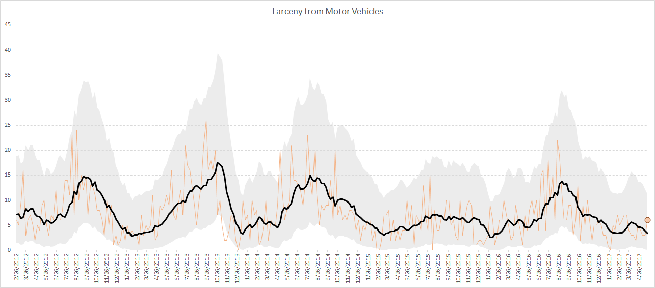
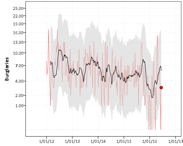
In the weekly chart the red line is the actual data, the black line is the average of the prior 8 weeks, and the grey band is a Poisson confidence interval around that prior moving average. The red dot is the most recent week.

And we will also be making a monthly seasonal chart:

The red line is the counts of calls per month in the current year, and the lighter grey lines are prior years (here going back to 2012).


So to start, I saved the 2012 through currently 6/20/2016 calls for service data as a csv file. And here is the code to read in that incident level data.

*Change this to where the csv file is located on your machine.
FILE HANDLE data /NAME = "C:\Users\andrew.wheeler\Dropbox\Documents\BLOG\Tables_Graphs".
GET DATA  /TYPE=TXT
  /FILE="data\Calls_for_Service_Dashboard_data.csv"
  /ENCODING='UTF8'
  /DELCASE=LINE
  /DELIMITERS=","
  /QUALIFIER='"'
  /ARRANGEMENT=DELIMITED
  /FIRSTCASE=2
  /DATATYPEMIN PERCENTAGE=95.0
  /VARIABLES=
  AdjustedLatitude AUTO
  AdjustedLongitude AUTO
  AlcoholRelated AUTO
  Area AUTO
  CallDateTime AUTO
  CallType AUTO
  Domv AUTO
  DayofWeek AUTO
  DrugRelated AUTO
  EndDateTime AUTO
  GeneralTimeofDay AUTO
  IncidentNumber AUTO
  LocationType AUTO
  MentalHealthRelated AUTO
  MethodofEntry AUTO
  Month AUTO
  PointofEntry AUTO
  StartDateTime AUTO
  Street AUTO
  Team AUTO
  Year AUTO
  /MAP.
CACHE.
EXECUTE.
DATASET NAME CFS.

First I will be making the weekly chart. What I did when I was working as an analyst was make a chart that showed the recent weekly trends and to identify if the prior week was higher than you might expect it to be. The weekly patterns can be quite volatile though, so I smoothed the data based on the average of the prior eight weeks, and calculated a confidence interval around that average count (based on the Poisson distribution).

As a start, we are going to turn our date variable, CallDateTime, into an SPSS date variable (it gets read in as a string, AM/PM in date-times are so annoying!). Then we are going to calculate the number of days since some baseline – here it is 1/1/2012, which is Sunday. Then we are going to calculate the weeks since that Sunday. Lastly we select out the most recent week, as it is not a full week.

*Days since 1/1/2012.
COMPUTE #Sp = CHAR.INDEX(CallDateTime," ").
COMPUTE CallDate = NUMBER(CHAR.SUBSTR(CallDateTime,1,#Sp),ADATE10).
COMPUTE Days = DATEDIFF(CallDate,DATE.MDY(1,1,2012),"DAYS").
COMPUTE Weeks = TRUNC( (Days-1)/7 ).
FREQ Weeks /FORMAT = NOTABLE /STATISTICS = MIN MAX.
SELECT IF Weeks < 233.

Here I do weeks since a particular date, since if you do XDATE.WEEK you can have not full weeks. The magic number 233 can be replaced by sometime like SELECT IF Weeks < ($TIME - 3*24*60*60). if you know you will be running the syntax on a set date, such as when you do a production job. (Another way is to use AGGREGATE to figure out the latest date in the dataset.)

Next what I do is that when you use AGGREGATE in SPSS, there can be missing weeks with zeroes, which will mess up our charts. There end up being 22 different call-types in the Burlington data, so I make a base dataset (named WeekFull) that has all call types for each week. Then I aggregate the original calls for service dataset to CallType and Week, and then I merge the later into the former. Finally I then recode the missings intos zeroes.

*Make sure I have a full set in the aggregate.
FREQ CallType.
AUTORECODE CallType /INTO CallN.
*22 categories, may want to collapse a few together.
INPUT PROGRAM.
LOOP #Weeks = 0 TO 232.
  LOOP #Calls = 1 TO 22.
    COMPUTE CallN = #Calls.
    COMPUTE Weeks = #Weeks.
    END CASE.
  END LOOP.
END LOOP.
END FILE.
END INPUT PROGRAM.
DATASET NAME WeekFull.

*Aggregate number of tickets to weeks.
DATASET ACTIVATE CFS.
DATASET DECLARE WeekCalls.
AGGREGATE OUTFILE='WeekCalls'
  /BREAK Weeks CallN
  /CallType = FIRST(CallType)
  /TotCalls = N.

*Merge Into WeekFull.
DATASET ACTIVATE WeekFull.
MATCH FILES FILE = *
  /FILE = 'WeekCalls'
  /BY Weeks CallN.
DATASET CLOSE WeekCalls.
*Missing are zero cases.
RECODE TotCalls (SYSMIS = 0)(ELSE = COPY).

Now we are ready to calculate our statistics and make our charts. First we create a date variable that represents the beginning of the week (for our charts later on.) Then I use SPLIT FILE and CREATE to calculate the prior moving average only within individiual call types. The last part of the code calculates a confidence interval around prior moving average, and assumes the data is Poisson distributed. (More discussion of this is in my academic paper.)

DATASET ACTIVATE WeekFull.
COMPUTE WeekBeg = DATESUM(DATE.MDY(1,1,2012),(Weeks*7),"DAYS").
FORMATS WeekBeg (ADATE8).

*Moving average of prior 8 weeks.
SORT CASES BY CallN Weeks.
SPLIT FILE BY CallN.
CREATE MovAv = PMA(TotCalls,8).
*Calculating the plus minus 3 Poisson intervals.
COMPUTE #In = (-3/2 + SQRT(MovAv)).
DO IF #In >= 0.
  COMPUTE LowInt = #In**2.
ELSE.
  COMPUTE LowInt = 0.
END IF.
COMPUTE HighInt = (3/2 + SQRT(MovAv))**2.
EXECUTE.

If you rather use the inverse of the Poisson distribution I have notes in the code at the end to do that, but they are pretty similar in my experience. You also might consider (as I mention in the paper), rounding fractional values for the LowInt down to zero as well.

Now we are ready to make our charts. The last data manipulation is to just put a flag in the file for the very last week (which will be marked with a large red circle). I use EXECUTE before the chart just to make sure the variable is available. Finally I keep the SPLIT FILE on, which produces 22 charts, one for each call type.

IF Weeks = 232 FinCount = TotCalls.
EXECUTE.

*Do a quick look over all of them.
GGRAPH
  /GRAPHDATASET NAME="graphdataset" VARIABLES=WeekBeg TotCalls MovAv LowInt HighInt FinCount MISSING=VARIABLEWISE
  /GRAPHSPEC SOURCE=INLINE.
BEGIN GPL
  SOURCE: s=userSource(id("graphdataset"))
  DATA: WeekBeg=col(source(s), name("WeekBeg"))
  DATA: TotCalls=col(source(s), name("TotCalls"))
  DATA: MovAv=col(source(s), name("MovAv"))
  DATA: LowInt=col(source(s), name("LowInt"))
  DATA: HighInt=col(source(s), name("HighInt"))
  DATA: FinCount=col(source(s), name("FinCount"))
  SCALE: pow(dim(2), exponent(0.5))
  GUIDE: axis(dim(1))
  GUIDE: axis(dim(2), label("Crime Count"))
  ELEMENT: line(position(WeekBeg*TotCalls), color(color.red), transparency(transparency."0.4"))
  ELEMENT: area(position(region.spread.range(WeekBeg*(LowInt+HighInt))), color.interior(color.lightgrey), 
  transparency.interior(transparency."0.4"), transparency.exterior(transparency."1"))
  ELEMENT: line(position(WeekBeg*MovAv))
  ELEMENT: point(position(WeekBeg*FinCount), color.interior(color.red), size(size."10"))
END GPL.
SPLIT FILE OFF.

This is good for the analyst, I can monitor many series. Here is an example the procedure produces for mental health calls:

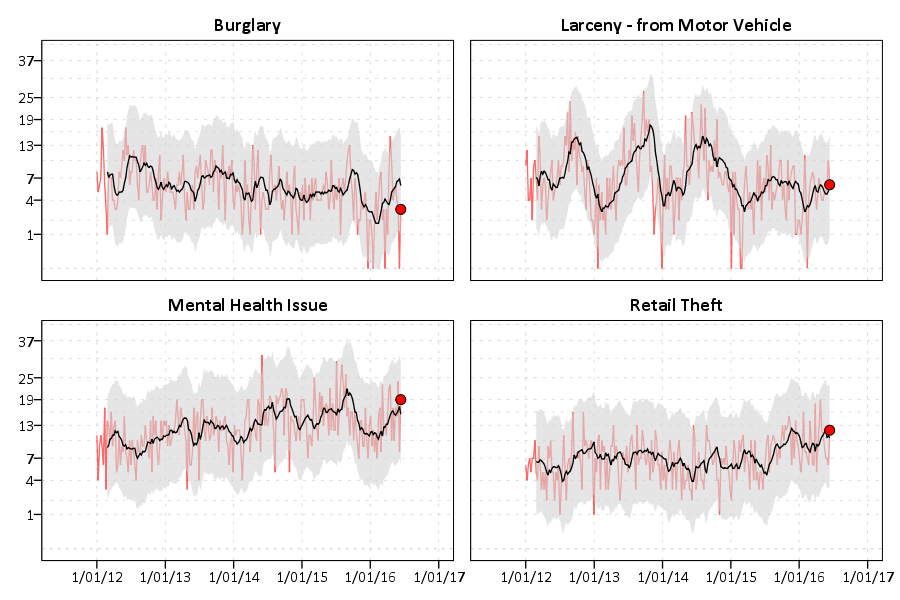
The current value is within the confidence band, so it is not alarmingly high. But we can see that they have been trending up over the past few years. Plotting on the square root scale makes the Poisson count data have the same variance, but a nice thing about the SPLIT FILE approach is that SPSS does smart Y axis ranges for each individual call type.

You can update this to make plots for individual crimes, and here I stuff four different crime types into a small multiple plot. I use a TEMPORARY and SELECT IF statement before the GGRAPH code to select out the crime types I am interested in.

FORMATS TotCalls MovAv LowInt HighInt FinCount (F3.0).
TEMPORARY.
SELECT IF ANY(CallN,3,10,13,17).
GGRAPH
  /GRAPHDATASET NAME="graphdataset" VARIABLES=WeekBeg TotCalls MovAv LowInt HighInt FinCount CallN MISSING=VARIABLEWISE
  /GRAPHSPEC SOURCE=INLINE.
BEGIN GPL
  PAGE: begin(scale(900px,600px))
  SOURCE: s=userSource(id("graphdataset"))
  DATA: WeekBeg=col(source(s), name("WeekBeg"))
  DATA: TotCalls=col(source(s), name("TotCalls"))
  DATA: MovAv=col(source(s), name("MovAv"))
  DATA: LowInt=col(source(s), name("LowInt"))
  DATA: HighInt=col(source(s), name("HighInt"))
  DATA: FinCount=col(source(s), name("FinCount"))
  DATA: CallN=col(source(s), name("CallN"), unit.category())
  COORD: rect(dim(1,2), wrap())
  SCALE: pow(dim(2), exponent(0.5))
  GUIDE: axis(dim(1))
  GUIDE: axis(dim(2), start(1), delta(3))
  GUIDE: axis(dim(3), opposite())
  GUIDE: form.line(position(*,0),color(color.lightgrey),shape(shape.half_dash))
  ELEMENT: line(position(WeekBeg*TotCalls*CallN), color(color.red), transparency(transparency."0.4"))
  ELEMENT: area(position(region.spread.range(WeekBeg*(LowInt+HighInt)*CallN)), color.interior(color.lightgrey), 
  transparency.interior(transparency."0.4"), transparency.exterior(transparency."1"))
  ELEMENT: line(position(WeekBeg*MovAv*CallN))
  ELEMENT: point(position(WeekBeg*FinCount*CallN), color.interior(color.red), size(size."10"))
  PAGE: end()
END GPL.
EXECUTE.

You could do more fancy time-series models to create the confidence bands or identify the outliers, (exponential smoothing would be similar to just the prior moving average I show) but this ad-hoc approach worked well in my case. (I wanted to make more fancy models, but I did not let the perfect be the enemy of the good to get at least this done when I was employed as a crime analyst.)


Now we can move onto making our monthly chart. These weekly charts are sometimes hard to visualize with highly seasonal data. So what this chart does is gives each year a new line. Instead of drawing error bars, the past years data show the typical variation. It is then easy to see seasonal ups-and-downs, as well as if the latest month is an outlier.

Getting back to the code — I activate the original calls for service database and then close the Weekly database. Then it is much the same as for weeks, but here I just use calendar months and match to a full expanded set of calls types and months over the period. (I do not care about normalizing months, it is ok that February is only 28 days).

DATASET ACTIVATE CFS.
DATASET CLOSE WeekFull.

COMPUTE Month = XDATE.MONTH(CallDate).
COMPUTE Year = XDATE.YEAR(CallDate).

DATASET DECLARE AggMonth.
AGGREGATE OUTFILE = 'AggMonth'
  /BREAK Year Month CallN
  /MonthCalls = N.

INPUT PROGRAM.
LOOP #y = 2012 TO 2016.
  LOOP #m = 1 TO 12.
    LOOP #call = 1 TO 22.
      COMPUTE CallN = #call.
      COMPUTE Year = #y.
      COMPUTE Month = #m.
      END CASE.
    END LOOP.
  END LOOP.
END LOOP.
END FILE.
END INPUT PROGRAM.
DATASET NAME MonthAll.

MATCH FILES FILE = *
  /FILE = 'AggMonth'
  /BY Year Month CallN.
DATASET CLOSE AggMonth.

Next I select out the most recent month of the date (June 2016) since it is not a full month. (When I originally made these charts I would normalize to days and extrapolate out for my monthly meeting. These forecasts were terrible though, even only extrapolating two weeks, so I stopped doing them.) Then I calculate a variable called Current – this will flag the most recent year to be red in the chart.

COMPUTE MoYr = DATE.MDY(Month,1,Year).
FORMATS MoYr (MOYR6) Year (F4.0) Month (F2.0).
SELECT IF MoYr < DATE.MDY(6,1,2016).
RECODE MonthCalls (SYSMIS = 0)(ELSE = COPY).

*Making current year red.
COMPUTE Current = (Year = 2016).
FORMATS Current (F1.0).

SORT CASES BY CallN MoYr.
SPLIT FILE BY CallN.

*Same thing with the split file.
GGRAPH
  /GRAPHDATASET NAME="graphdataset" VARIABLES=Month MonthCalls Current Year
  /GRAPHSPEC SOURCE=INLINE.
BEGIN GPL
  SOURCE: s=userSource(id("graphdataset"))
  DATA: Month=col(source(s), name("Month"), unit.category())
  DATA: MonthCalls=col(source(s), name("MonthCalls"))
  DATA: Current=col(source(s), name("Current"), unit.category())
  DATA: Year=col(source(s), name("Year"), unit.category())
  GUIDE: axis(dim(1))
  GUIDE: axis(dim(2), label("Calls"), start(0))
  GUIDE: legend(aesthetic(aesthetic.color.interior), null())
  SCALE: cat(aesthetic(aesthetic.color.interior), map(("0",color.lightgrey),("1",color.red)))
  ELEMENT: line(position(Month*MonthCalls), color.interior(Current), split(Year))
END GPL.

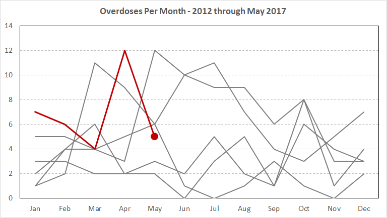
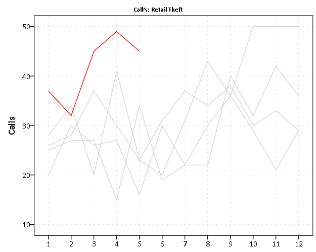
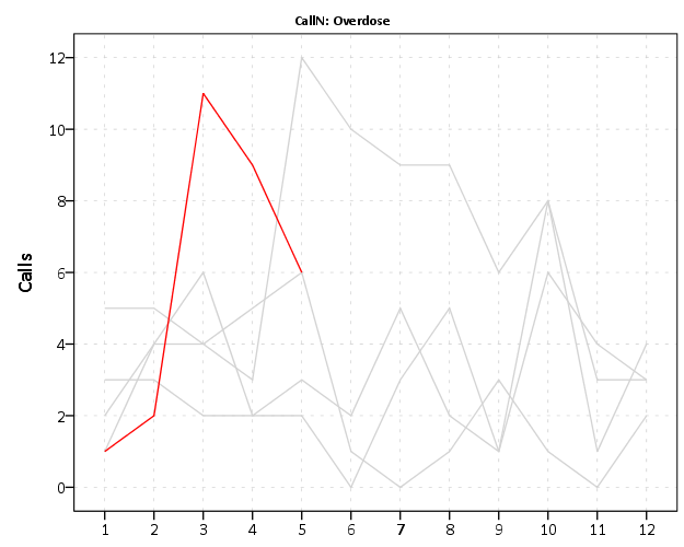
You can again customize this to be individual charts for particular crimes or small multiples. You can see in the example at the beginning of the post Retail thefts are high for March, April and May. I was interested to examine overdoses, as the northeast (and many parts of the US) are having a problem with heroin at the moment. In the weekly charts they are so low of counts it is hard to see any trends though.

We can see that overdoses were high in March. The other highest line are months in 2015, so it looks like a problem here in Burlington, but it started around a year ago.

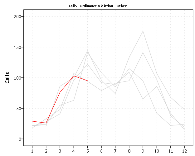
For low counts of crime (say under 20 per month) seasonality tends to be hard to spot. For crimes more frequent though you can often see pits and peaks in summer and winter. It is not universal that crimes increase in the summer though. For ordinance violations (and ditto for Noise complaints) we can see a pretty clear peak in September. (I don’t know why that is, there is likely some logical explanation for it though.)

My main motivation to promote these is to replace terrible CompStat tables of year-over-year percent changes. All of these patterns I’ve shown are near impossible to tell from tables of counts per month.

Finally if you want to export your images to place into another report, you can use:

OUTPUT EXPORT /PNG IMAGEROOT = "data\TimeGraphs.png".

PNG please – simple vector graphics like these should definately not be exported as jpegs.

Here is a link to the full set of syntax and the csv data to follow along. I submitted to doing an hour long training session at the upcoming IACA conference on this, so hopefully that gets funded and I can go into this some more.

Using and Making Cumulative Probability Charts

Stephen Few had a recent post critiquing an evaluation of a particular data visualization. Long story short, the experiment asked questions like “What is the probability that X is above 5?”, and showed the accuracy based on mean+error bar charts, histogram like visualizations, and animated vizualations showing random draws.

It is always the case in data viz. that some charts are easier to answer particular questions. This is one question, what is the probability a value is above X, in which traditional histograms or error bar charts are not well suited for. But there is an alternative I don’t see used very often, the cumulative probability chart, that is well suited to answer that question.

It is a totally reasonable question to ask as well. For one example use when I was a crime analyst, I used this chart to show the time in-between shootings. Many shootings are retaliatory so I was interested in saying if a shooting happened on Sunday, how long should be PD be on guard for after an initial shooting. Do most retaliatory shootings happen within hours, days, or weeks of a prior shooting? This is a hard question to answer with histograms, but is easier to answer with cumulative probability plots.

Here is that example chart for time-in-between shootings:

Although this chart is not regularly used, it is really easy to explain how to interpret. For example, at time equals 7 days (on the X axis), the probability that a shooting would have occurred is under 60%. In my opinion, it is easier to explain this chart than a histogram to a lay audience.

To produce the chart it is often not a canned option in software, but it takes very simple set of steps to produce the right ingrediants – and then you can use a typical line chart. So those steps generically are:

  • sort the data
  • rank the data (1 for the lowest value, 2 for the second lowest value, etc.)
  • calculate rank/(total sample size) – call this Prop
  • plot the data on the X axis, and Prop on the Y axis

Which can be easily done in any software, but here you can download an excel spreadsheet here used to make the above chart.

A variant of this chart often used in crime analysis is the proportion of places on the X axis and the cumulative proportion of crime on the Y axis. E.g. Pareto’s 80/20 rule – or 50/1 rule – or whatever. The chart makes it easy to pick whatever cut-offs you want. If you have your spatial units of analysis in one column, and the total number of crimes in a second column, the procedure to produce this chart is:

  • sort the data descending by number of crimes
  • rank the data
  • calculate rank/(total sample size) – this equals the proportion of all spatial units – call this PropUnits
  • calculate the cumulative number of crimes – call this Cum_Crime
  • calculate Cum_Crime/(Total Crime) – this equals the proportion of all crimes – call this PerCumCrime
  • plot PerCumCrime on the Y axis and PropUnits on the X axis.

See the third sheet of the excel file for a hypothetical example. This pattern basically happens in all aspects of criminal justice. That is, the majority of the bad stuff is happening among a small number of people/places. See this example from William Spelman showing places, victims, and offenders.

We can see there that 10% of the victims account for 40% of all victimizations etc.

Testing day-of-week crime randomness paper published

My paper, Testing Serial Crime Events for Randomness in Day of Week Patterns with Small Samples, was recently published in the Journal of Investigative Pyschology and Offender Profiling. Here is the pre-print version on SSRN if you can’t get access to that journal.

The main idea behind the paper was if you had a series of a few crime events that you know are linked to the same offender, can we tell if those patterns are random with respect to the day of the week? We know spatial patterns are often clustered, but police responses such as surveillance are conditioned not only on a spatial location, but take place during certain days and times. I wanted to know when I could go to command staff and say, yeah you should BOLO on Saturday. Or just as importantly say in response, no the observed patterns could easily happen if the offender were just randomly picking days.

In the paper I show that if you have only 3 events and they all occur on the same day, you would reject the null that crimes have an equal probability across all seven days of the week at a p-value of less than 0.05. I also show that the exact test I propose has pretty good power for as few as 8 events in the series. So if you have, say 10 events and you fail to reject the null that each day of the week has equal probability of being chosen, it is pretty good evidence that a police response should not have any preference for a particular day.

To illustrate how one would use the test, I have a simple spreadsheet posted here (in the zip file has my other SPSS code to reproduce the results in the paper) in which you can type in the days of the week that the crimes are occurring on, and it calculates the hypothesis test.

The spreadsheet contains both the G-test and Kuiper’s V test. If you don’t read the paper and understand the difference, just use the G-test and ignore the Kuiper’s V results. For crime analysts, this is basically the minimum of what you need to know.


For analysts who are more into the nitty gritty, I also have some R code that is a bit more flexible, and calculates the exact test for varying numbers of bins and provides some code to conduct power analysis. So you can either download the code from GitHub and insert it to define the functions, or simply copy-paste it into the console. The only library dependency is the partitions library, so make sure that is installed before following along.

So if you have downloaded the code, you can use something like below to insert the functions and load the partitions library.

library(partitions)
mydir <- "C:\\Users\\andrew.wheeler\\Dropbox\\Documents\\BLOG\\ExactTest_Weekdays"
setwd(mydir)
source("Exact_Dist.R")

Now, say you had a series of crimes that had 4 on Saturday, 3 on Tuesday, and 1 on Sunday. You can test this for randomness by simply using:

crime <- c(1,0,3,0,0,0,4)
res <- SmallSampTest(d=crime)
res

Which prints at the console:

Small Sample Test Object 
Test Type is G 
Statistic is 15.5455263389754 
p-value is:  0.0182662  
Data are:  1 0 3 0 0 0 4 
Null probabilities are:  0.14 0.14 0.14 0.14 0.14 0.14 0.14 
Total permutations are:  3003  

This defaults to using the likelihood ratio G-test, but you can also use Kuiper’s V, the chi-square test, or the Komolgrov-Smirnov test. Also you can change the null hypothesis to not equal probability in the bins. I default to the G-test in my paper because it is more powerful than the more typical chi-square after 8 crimes for 7 day-of-week bins, but equal in power to the chi-square for smaller sample sizes. So to do the chi-square test on the same data, use:

resChi <- SmallSampTest(d=crime, type="Chi")
resChi
chisq.test(crime) #for comparison to base R 
chisq.test(crime, simulate.p.value = TRUE, B = 10000)

Which you can see the test statistic mimics base R’s chisq.test, and the p-value is slightly higher than the asymptotic p-value (the exact test should always have a higher p-value than the asympotic distribution, and here it is lower than the simulated p-value). This situation the simulation approach would have been fine. I prefer the exact approach when feasible though, because it is exact, and you don’t need to worry about convergence for the simulation (which most everyone simply picks a large number and hopes for the best).

I’ve also made some code that allows for easy evaluation of the power of the exact test. Coding wise it was easiest to simply use the original object created with the test, so I know it invites post-hoc power analysis – forgive me for my slothness in coding practices. So say you wanted to do apriori power analysis with the Kuiper’s V test for 10 bins and 15 observations (so over 1.3 million permutations, i.e. n <- 15; m <- 10; choose(n+m-1,m-1)). You can simply make an original object (with any observed values across the bins).

test10_data <- c(15,rep(0,9))
test10_perm <- SmallSampTest(d=test10_data, type="KS")
#takes around a minute

The default null is equal probability across the bins, and to do a power analysis you have to specify an alternative. Lets say for the alternative there is equal probability in 5 of the bins, and zero probability in the other 5. (Most of the work is done in making the original permutation object, the power analysis is quite fast, hence why I coded it to work this way.)

p_alt <- c(rep(1/5,5),rep(0,5))
Pow_test <- PowAlt(SST=test10_perm,p_alt=p_alt)
Pow_test

This prints out at the console:

Power for Small Sample Test 
Test statistic is: KS  
Power is: 0.1822815  
Null is: 0.1 0.1 0.1 0.1 0.1 0.1 0.1 0.1 0.1 0.1  
Alt is: 0.2 0.2 0.2 0.2 0.2   0   0   0   0   0  
Alpha is: 0.05  
Number of Bins: 10  
Number of Observations: 15  

So for this alternative there is quite low power, only 0.18. But if we change it to only have mass in four of the bins, the power goes way up to over 0.99.

> p_alt2  Pow_test2  Pow_test2
Power for Small Sample Test 
Test statistic is: KS  
Power is: 0.9902265  
Null is: 0.1 0.1 0.1 0.1 0.1 0.1 0.1 0.1 0.1 0.1  
Alt is: 0.25 0.25 0.25 0.25   0   0   0   0   0   0  
Alpha is: 0.05  
Number of Bins: 10  
Number of Observations: 15 

So this shows how the exact test R code can be extended beyond just 7 day-of-week bins. I have not done really any exploration of the power of the KS test or differing numbers of bins though.

The spatial clustering of hits-vs-misses in shootings using Ripley’s K

My article, Replicating Group-Based Trajectory Models of Crime at Micro-Places in Albany, NY was recently published online first at the Journal of Quantitative Criminology (here is a pre-print version, and you can get my JQC offprint for the next few weeks).

Part of the reason I blog is to show how to replicate some of my work. I have previously shown how to generate the group based trajectory models (1,2), and here I will illustrate how to replicate some of the point pattern analysis I conducted in that paper.

A regular task for an analyst is to evaluate spatial clustering. A technique I use in that article is to use Ripley’s K statistic to evaluate clustering between different types of events, or what spatial statistics jargon calls a marked point pattern. I figured I would illustrate how to do this on some example point patterns of shootings, so analysts could replicate for other situations. The way crime data is collected and geocoded makes generating the correct reference distributions for the tests different than if the points could occur anywhere in the study region.

An example I am going to apply are shooting incidents that have marks of whether they hit the intended victim or missed. One theory in criminology is that murder is simply the extension of general violence — with the difference in aggravated assault versus murder often being happenstance. One instance this appears to be the case from my observations are shootings. It seems pure luck whether an individual gets hit or the bullets miss everyone. Here I will see if there appear to be any spatial patterning in shots fired with a victim hit. That is, we know that shootings themselves are clustered, but within those clusters of shootings are the locations of hits-and-misses further clustered or are they random?

A hypothetical process in which clustering of shooting hits can occur is if some shootings are meant to simply scare individuals vs. being targeted at people on the street. It could also occur if there are different tactics, like drive-bys vs. being on foot. This could occur if say one area had many shootings related to drug deals gone wrong, vs. another area that had gang retaliation drive by shootings. If they are non-random, the police may consider different interventions in different places – probably focusing on locations where people are more likely to be injured from the shooting. If they are random though, there is nothing special about analyzing shootings with a person hit versus shootings that missed everyone – you might as well analyze and develop strategy for all shootings.

So to start we will be using the R statistical package and the spatstat library. To follow along I made a set of fake shooting data in a csv file. So first load up R, I then change the working directory to where my csv file is located, then I read in the csv into an R data frame.

library(spatstat)

#change R directory to where your file is
MyDir <- "C:\\Users\\andrew.wheeler\\Dropbox\\Documents\\BLOG\\R_shootingVic\\R_Code"
setwd(MyDir)

#read in shooting data
ShootData <- read.csv("Fake_ShootingData.csv", header = TRUE)
head(ShootData)

The file subsequently has four fields, ID, X & Y coordinates, and a Vic column with 0’s and 1’s. Next to conduct the spatial analysis we are going to convert this data into an object that the spatstat library can work with. To do that we need to create a study window. Typically you would have the outline of the city, but for this analysis the window won’t matter, so here I make a window that is just slightly larger than the bounding box of the data.

#create ppp file, window does not matter for permuation test
StudyWin <- owin(xrange=c(min(ShootData$X)-0.01,max(ShootData$X)+0.01),yrange=c(min(ShootData$Y)-0.01,max(ShootData$Y)+0.01))
Shoot_ppp <- ppp(ShootData$X, ShootData$Y, window=StudyWin, marks=as.factor(ShootData$Vic), unitname = c("meter","meters"))

Traditionally when Ripley’s K was originally developed it was for points that could occur anywhere in the study region, such as the location of different tree species. Crimes are a bit different though, in that there are some areas in any city that a crime basically cannot occur (such as the middle of a lake). Also, crimes are often simply geocoded according to addresses and intersections, so this further reduces the locations where the points can be located in a crime dataset. To calculate the sample statistic for Ripley’s K one does not need to account for this, but to tell whether those patterns are random one needs to simulate the point pattern under a realistic null hypothesis. There are different ways to do the simulation, but here the simulation keeps the shooting locations fixed, but randomly assigns a shooting to be either a victim or a not with the same marginal frequencies. That is, it basically just shuffles which events are counted as a victim being hit or one in which there were no people hit. The Dixon article calls this the random relabelling approach.

Most of the spatstat functions can take a separate list of point patterns to use to simulate error bounds for different functions, so this function takes the initial point pattern, generates the permutations, and stuffs them in a list. I set the seed so the analysis can be reproduced exactly.

#generate the simulation envelopes to use in the Cross function
MarkedPerms <- function(ppp, nlist) {
  require(spatstat)
  myppp_list <- c() #make empty list
  for (i in 1:nlist) {
    current_ppp <-  ppp(ppp$x, ppp$y,window=ppp$window,marks=sample(ppp$marks))  #making permutation      
    myppp_list[[i]] <- current_ppp                                               #appending perm to list
  }
  return(myppp_list)
}

#now making a set of simulated permutations
set.seed(10) #setting seed for reproducibility
MySimEvel <- MarkedPerms(ppp=Shoot_ppp,nlist=999)

Now we have all the ingredients to conduct the analysis. Here I call the cross K function and submit my set of simulated point patterns named MySimEvel. With only 100 points in the dataset it works pretty quickly, and then we can graph the Ripley’s K function. The grey bands are the simulated K statistics, and the black line is the observed statistic. We can see the observed is always within the simulated bands, so we conclude that conditional on shooting locations, there is no clustering of shootings with a victim versus those with no one hit. Not surprising, since I just simulated random data.

#Cross Ripleys K
CrossK_Shoot <- alltypes(Shoot_ppp, fun="Kcross", envelope=TRUE, simulate=MySimEvel)
plot(CrossK_Shoot$fns[[2]], main="Cross-K Shooting Victims vs. No Victims", xlab="Meters")

I conducted this same analysis with actual shooting data in three separate cities that I have convenient access to the data. It is a hod podge of length, but City A and City B have around 100 shootings, and City C has around 500 shootings. In City A the observed line is very near the bottom, suggesting some evidence that shootings victims may be further apart than would be expected, but for most instances is within the 99% simulation band. (I can’t think of a theoretical reason why being spread apart would occur.) City B is pretty clearly within the simulation band, and City C’s observed pattern mirrors the mean of the simulation bands almost exactly. Since City C has the largest sample, I think this is pretty good evidence that shootings with a person hit are spatially random conditional on where shootings occur.

Long story short, when conducting Ripley’s K with crime data, the default way to generate the simulation envelopes for the statistics are not appropriate given how crime data is recorded. I show here one way to account for that in generating simulation envelopes.

Some ad-hoc fuzzy name matching within Police databases

A repeated annoying task I have had to undertake is take a list of names and date-of-births and match them to a reference set. This can happen when you try to merge data from different sources. Or when working with police RMS data, a frequent problem is the same individual can go into the master name list multiple times. This can be either due to data error, or someone being malicious and providing the PD with fraudulent data.

Most often I am trying to match a smaller set of names to a bigger set from a police RMS system. Typically what I do is grab all of the names in the police RMS, make them the same case, and then simply sort the file by last then first name. Then I typically go through one by one from the smaller file and identify the name ID’s that are in the sorted bigger police database. Ctrl-F can make it a quick search for only a few people.

This works quite well for small numbers, but I wanted to see if I could make some simple rules when I need to match a larger list. For example, the above workflow may be fine if I need to look up 10 names quickly, but say you want to eliminate duplicates in the entire PD RMS system? A manually hand search through 100,000+ names is crazy (and will be out of date before you finish).

A tool I’ve used in the past (and would recommend) is FRIL, Fine-grained records integration and linkage tool. In a nutshell the way that tool works is that you can calculate string distances between names and/or date distances between date-of-births from two separate files. Then you specify how close you want the records to be to either automatically match the records or manually view and make a personal determination if the two records are the same person. FRIL has a really great interface to quickly view the suggested matches and manually confirm or reject certain matches.

FRIL uses the Potter Stewart I know it when I see it approach to finding matches. There is no ground truth, you just use your best judgement whether two names belong to the same person, and FRIL uses some metrics to filter out the most unlikely candidates. I have a bit of a unique strategy though to identify typical string and date of birth differences in fuzzy name matches by using Police RMS data itself. Police RMS’s tend to have a variety of people who are linked up to the same master name index value, but for potentially several reasons they have various idiosyncrasies among different individual incidents. This allows me to calculate distances within persons, so a ground truth estimate, and then I can evaluate different distances compared to a control sample to see how well they the metrics discriminate matches.

There can be several reasons for slightly different data among an individuals incidents in a police RMS, but that they end up being linked to the same person. One is that frequently RMS systems incorporate tables from several different data sources, dispatchers have their own CAD system, the PD has a system to type in paper records, custodial arrests/finger printing may have another system, etc. Merging this data into one RMS may simply cause differences in how the data is stored or even how particular fields tend to be populated in the database. A second reason is that individuals can be ex-ante associated to a particular master name index, but can still have differences is various person fields for any particular incident.

One simple example is that for an arrest report the offender may have an old address in the system, so the officer types in the new address. The same thing can happen to slight name changes or DOB changes. The master name index should update with the most recent info, but you have a record trail of all the minor variations through each incident. Depending on the type of involvement in an incident has an impact on what information is collected and the quality of that information as well. For example, if I was interviewed as a witness to a crime, I may just go down in the report as Andy Wheeler with no date of birth info. If I was arrested, someone would take more time to put in my full name, Andrew Wheeler, and my date of birth. But if the original person inputting the data took the time, they would probably realize I was the same person and associate me with the same master ID.

So I can look at these within ID changes to see the typical distances. What I did was take a name database from a police department I work with, make all pair-wise comparisons between unique names and date of births, and then calculate several string distances between the names and the date differences between listed DOB’s. I then made a randomly matched sample for a comparison group. For the database I was working with this ended up being over 100,000 people with the same ID, but different names/DOB’s somewhere in different incidents, with an average of between 2~3 different names/dob’s per person (so a sample of nearly 200,000 same name comparisons, two names only results in one comparison, but three names results in 3 comparisons). My control sample took one of these names person and matched another random person in the database as a control group, so I have a control group sample of over 100,000 cases.

The data I was working with is secondary, so the names were already aggregated to Last, First Middle. If I had the original database I could do distances for the individual fields (and probably not worry about the middle name) but it somewhat simplifies the analysis as well. Here are some histograms of the Levenshtein distance between the name strings for the same person and random samples. The Levenshtein distance is the number of single edits it takes to transform one string to another string, so 0 would be the same word.

Part of the reason the distances within the same name have such a long tail is because of the already aggregated data. There end up being some people with full middle names, some with middle initials, and some with no middle names at all. So what I did was calculate a normalized Levenshtein distance based on the max and min possible values (listed at the Wikipedia page) the string can take given the size of the two input strings. The minimum value is the difference in the length of the two strings, the maximum is the length of the longest string. So then I calculate NormLevenDist = (LevenDist - min)/(max - min). This would cause Wheeler, Andy P and Wheeler, Andy Palmer to have a normalized distance of zero, whereas the edit distance would be 5. So in these histograms you can see even more discrimination between the two classes, based mainly on such names being perfect subsets of other names.

If you eliminate the 0’s in the normalized distance, you can get a better look at the shapes of each distribution. There is no clear cut-off between the samples, but there is a pretty clear difference in the distributions.

I also calculated the Jaro-Winkler and the Dice (bi-gram) string distances. All four of these metrics had a fairly high correlation, around 0.8 with one another, and all did pretty well classifying the same ID’s according to their ROC curves.

If I wanted to train a classifier as accurately as possible, I would use all of these metrics and probably make some sort of decision tree (or estimate their effects via logistic regression), but I wanted to make a simple function (since it will be doing quite a few comparisons) that calculates as few of the metrics as possible, so I just went with the normalized Levenshtein distance here. Jaro-Winkler would probably be more competitive if I had the separate first and last names (and played around with the weights for the beginning and ends of the strings). If you had mixed strings, like some are First Middle Last and others are Last First I suspect the dice similarity would be the best.

But in the end I think all of the string metrics will do a pretty similar job for this input data, and the normalized Levenshtein distance will work pretty well so I am going to stick with that. (I don’t consider soundex matching here, I’ve very rarely come across an example where soundex would match but had a high edit distance for names, e.g. typos are much more common than intentional mis-spellings based on enunciation I believe, and even the intentional mis-spellings tend to have a small edit distance.)

Now looking at the absolute differences in the DOB’s (where both are available) provides a bit of a different pattern. Here is the histograms

But I think the easiest illustration of this is to examine the frequency table of the most common day differences for the same individuals.

Obviously zero is the most common, but you can see a few other bumps that illustrate the nature of data mistakes. The second is 365 days – exactly off by one year. Also in the top 10 are 366, 731 & 730 – off by either a year and a day or two years. 1096, 1095, 1461, 1826, are examples of these yearly cycles as well. 36,525 are examples of being off by a century! Somewhere along the way some of the DOB fields were accidentally assigned to dates in the future (such as 2032 vs. 1932). The final examples are off by some other number typical of a simple typo, such as 10, 20, or by the difference in one month 30,31,27. By the end of this table of PDF of the same persons is smaller than the PDF of the control sample.

I also calculated string distances by transforming the DOB’s to mm/dd/yy format, but when incorporating the yearly cycles and other noted mistakes they did not appear to offer any new information.

So based on this information, I made a set of ad-hoc rules to classify matched names. I wanted to keep the false positive rate at less than 1 in 1,000, but make the true positive as high as possible. The simple rules I came up with were:

  • If a normalized Levenshtein distance of less than 0.2, consider a match
  • If a normalized Levenshtein distance of less than 0.4 and a close date, consider a match.

Close dates are defined as:

  • absolute difference of within 10 days OR
  • days apart are 10,20,27,30,31 OR
  • the number of days within a yearly cycle are less than 10

This match procedure produces the classification table below:

The false positive rate is right where I wanted it to be, but the true positive is a bit lower than I hoped. But it is a simple tool though to implement, and built into it you can have missing data for a birthday.

It is a bit hard to share this data and provide reproducible code, but if you want help doing something similar with your own data just shoot me an email and I will help. This was all done in SPSS and Python (using the extended transforms python code). In the end I wanted to make a simple Python function to use with the FUZZY command to automatically match names.

Tables and Graphs paper rejection/update – and on the use of personal pronouns in scientific writing

My paper, Tables and Graphs for Monitoring Temporal Crime Patterns was recently rejected from Policing: An International Journal of Police Strategies & Management. I’ve subsequently updated the SSRN draft based on feedback from the review, and here I post the reviews and my responses to those reviews (in the text file).

One of the main critiques by both reviewers was that the paper was too informal, mainly because of the use of "I" in the paper. I use personal pronouns in writing intentionally, despite typical conventions in scientific writing, so I figured a blog post about why I do this is in order. I’ve been criticized for it on other occasions as well, but this is the first time it was listed as a main reason to reject an article of mine.

My main motivation comes from Michael Billig’s book Learn to Write Badly: How to Succeed in the Social Sciences (see a prior blog post I wrote on the contents). In a nut-shell, when you use personal pronouns it is clear that you, the author, are doing something. When you rewrite the sentence to avoid personal pronouns, you often obfuscate who the actor is in a particular sentence.

For an example of Billig’s point that personal pronouns can be more informative, I state in the paper:

I will refer to this metric as a Poisson z-score.

I could rewrite this sentence as:

This metric will be referred to as a Poisson z-score.

But that is ambiguous as to its source. Did someone else coin this phrase, and I am borrowing it? No – it is a phrase I made up, and using the personal pronoun clearly articulates that fact.

Pretty much all of the examples where I eliminated first person in the updated draft were of the nature,

In this article I discuss the use of percent change in tables.

which I subsequently changed to:

This article discusses the use of percent changes as a metric in tables.

Formal I suppose, but insipid. All rewriting the sentence to avoid the first person pronoun does is make the article seem like a sentient being, as well as forces me to use the passive tense. I don’t see how the latter is better in any way, shape, or form – yet this is one of the main reasons my paper is rejected above. The use of "we" in academic articles seems to be more common, but using "we" when there is only one author is just silly. So I will continue to use "I" when I am the only author.

Presentation at IACA 2015: An Exploratory Network Analysis of Hot People and Places

My work was accepted at the 2015 International Association of Crime Analysts Conference, so I will be going to Denver this fall to present. These are "NIJ Research Track" presentations, but basically took the place of the old MAPS conference presentations. So on Thursday at 2:30 (Panel 9) I will be presenting. The title of the presentation is An Exploratory Network Analysis of Hot People and Places, and below is the abstract for the talk:

Intelligence led policing practices focus on chronic offenders and hot spots of crime. I examine the connections between these hot people and hot places by considering micro places (street segments and intersections) and people as nodes in an interconnected network. I focus on whether hot people tend to have a finite set of locations they congregate, and whether hot places have unique profiles of chronic offenders. The end goal is to identify if observed patterns can help police combine targeted enforcement of hot people and hot places in one overarching strategy.

This is still a work in progress, but here is a quick preview. This graph is a random sample of offender footprints in each panel.

Also during this slot there are two other presentations, below is their info:

Title: Offender Based Investigations: A Paradigm Shift in Policing, Author: Chief James W. Buie, Gaston County Police

Abstract: Routine activity theory and research conducted by Wiles, P & Costello, A. (2000) ‘The Road to Nowhere’ prove criminals 1) commit crimes where comfortable and 2) are very likely to re-offend. Therefore it makes sense to elevate the importance of offender locations in relation to crimes. Our focus on the offender is called Offender Based Investigations (OBI). We’re using GIS to plot not only crimes but criminals as well. Our experience over the past seven years of utilizing OBI has proven that mapping offenders plays a critical role in solving crimes.

Title: A Spatial Network Analysis of Gangs Author: Davin Hall, Crime Analysis Specialist for the Greensboro PD

Abstract: Gangs are characterized by the associations between members and the territory that members operate in. Many representations of gang territory and gang networks are separate from one another; a map shows the territory while a network map shows linkages between individuals. This presentation demonstrates the combination of territory and network within a single map, for both gangs and gang members. This analysis shows law enforcement a clearer picture of the complex relationships that occur between and within gangs.

You can see the full agenda here. I really enjoyed the presentations last year at Seattle, and this year looks great as well. If you want any more info. on my particular work feel free to send me an email, or if you want to get together at Denver this fall.