How arrests reduce near repeats: Breaking the Chain paper published

My paper (with colleagues Jordan Riddell and Cory Haberman), Breaking the chain: How arrests reduce the probability of near repeat crimes, has been published in Criminal Justice Review. If you cannot access the peer reviewed version, always feel free to email and I can send an offprint PDF copy. (For those not familiar, it is totally OK/legal for me to do this!) Or if you don’t want to go to that trouble, I have a pre-print version posted here.

The main idea behind the paper is that crimes often have near-repeat patterns. That is, if you have a car break in on 100 1st St on Monday, the probability you have another car break in at 200 1st St later in the week is higher than typical. This is most often caused by the same person going and committing multiple offenses in a short time period. So a way to prevent that would on its face be to arrest the individual for the initial crime.

I estimate models showing the reduction in the probability of a near repeat crime if an arrest occurs, based on publicly available Dallas PD data (paper has links to replication code). Because near repeat in space & time is a fuzzy concept, I estimate models showing reductions in near repeats for several different space-time thresholds.

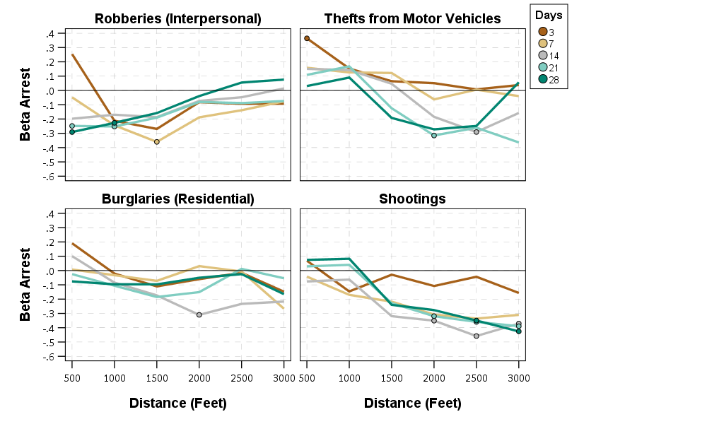
So here the model is Prob[Future Crime = I(time < t & distance < d)] ~ f[Beta*Arrest + sum(B_x*Control_x)] where the f function is a logistic function, and I plot the Beta estimates given different time and space look aheads. Points indicate statistical significance, so you can see they tend to be negative for many different crime and different specifications (with a linear coefficient of around -0.3).

Part of the reason I pursued this is that the majority of criminal justice responses to near repeat patterns in the past were target hardening or traditional police patrol. Target hardening (e.g. when a break in occurs, go to the neighbors and tell them to lock their doors) does not appear to be effective, but traditional patrol does (see the work of Rachel/Robert Santos for example).

It seems to me ways to increase arrest rates for crimes is a natural strategy that is worthwhile to explore for police departments. Easier said than done, but one way may be to prospectively identify incidents that are likely to spawn near repeats and give them higher priority in assigning detectives. In many urban departments, lower level property crimes are never assigned a detective at all.

Open Data and Reproducible Criminology Research

This is part of a special issue put together by Jonathan Grubb and Grant Drawve on spatial approaches to community violence. Jon and Grant specifically asked contributors to discuss a bit about open data standards and replication materials. I repost my thoughts on that here in full:

In reference to reproducibility of the results, we have provided replication materials. This includes the original data sources collated from open sources, as well as python, Stata, and SPSS scripts used to conduct the near-repeat analysis, prepare the data, generate regression models, and graph the results. The Dallas Police Department has provided one of the most comprehensive open sources of crime data among police agencies in the world (Ackerman & Rossmo, 2015; Wheeler et al., 2017), allowing us the ability to conduct this analysis. But it also identifies one particular weakness in the data as well – the inability to match the time stamp of the occurrence of an arrest to when the crime occurred. It is likely the case that open data sources provided by police departments will always need to undergo periodic revision to incorporate more information to better the analytic potential of the data.

For example, much analysis of the arrest and crime relationship relies on either aggregate UCR data (Chamlin et al., 1992), or micro level NIBRS data sources (Roberts, 2007). But both of these data sources lack specific micro level geographic identifiers (such as census tract or addresses of the events), which precludes replicating the near repeat analysis we conduct. If however NIBRS were to incorporate address level information, it would be possible to conduct a wide spread analysis of the micro level deterrence effects of arrests on near repeat crimes across many police jurisdictions. That would allow much broader generalizability of the results, and not be dependent on idiosyncratic open data sources or special relationships between academics and police departments. Although academic & police practitioner relationships are no doubt a good thing (for both police and academics), limiting the ability to conduct analysis of key policing processes to the privileged few is not.

That being said, currently both for academics and police departments there are little to no incentives to provide open data and reproducible code. Police departments have some slight incentives, such as assistance from governmental bodies (or negative conditions for funding conditional on reporting). As academics we have zero incentives to share our code for this manuscript. We do so simply because that is a necessary step to ensure the integrity of scientific research. Relying on the good will of researchers to share replication materials has the same obvious disadvantage that allowing police departments to pick and choose what data to disseminate does – it can be capricious. What a better system to incentivize openness may look like we are not sure, but both academics and police no doubt need to make strides in this area to be more professional and rigorous.

The random distribution of near-repeat strings

One thing several studies that examine near-repeat patterns have looked at is the distribution of the string of near-repeats. So near-repeats sometimes result in only 2 cases connected, sometimes 3, sometimes 4, etc. Here is an example from a recent work on arsons (Turchan et al., 2018):

Cory Haberman and Jerry Ratcliffe were the first I noticed to do this in this paper (Jerry’s near-repeat calculator has the option to export the strings). It is also a similar idea to what Davies and Marchione did in this paper.

Looking at these strings of events has clear utility for crime analysts, as they have a high probability of being linked to the same offender(s). Building off of some prior work, I wrote some python code to see what the distribution of these strings would look like when you randomly permuted the times in the data (which is the same approach used to estimate the intervals in the near repeat calculator). Here is the data and code, which is an analysis of 14,184 thefts from motor vehicles in Dallas that occurred in 2015.

So first I breakdown the total number of near repeat strings according to within 1000 feet and 7 days of each other. I then conduct 99 random permutations to see how many strings might happen by chance even if there is no near-repeat phenomenon. Some near-repeats can simply happen by chance, especially in places where crime is more prevalent. A length of string 1 in the table means it is not a near repeat, and 10+ means the string has 10 or more events in it. The numbers are the number of chains (in the Turchan article parlance), so 1,384 2-length chains means it includes 2,768 crime events.

If you compare the observed to the bounds in the table, you can see there are fewer isolates (1 length) in the observed than permutation distribution, and more 2 and 3 string events. After that the higher level strings occur just as frequently in the observed data than in the random data, with the exception of 10+ are fewer, but not by much.

So this provides evidence of the boost hypothesis in this data, albeit many near-repeat strings are still likely to occur just by chance, and the differences are not uber large. A crime analyst may be more interested in the question though "if I have X events in a near-repeat string, should I look into the data more". The idea being that since 2-strings are not that rare it would probably be a waste of an analysts time to dig into all of the two-events. I don’t think this is the perfect way to make that decision, but here is a breakdown of the distribution of strings for the permutated data.

So isolates happen in the random data 86% of the time. 2-strings happen 8.7% of the time, 3-strings 2.6%, etc. Based on this I would recommend that there needs to be at least 3 strings of near-repeat events if you have a low threshold in terms of "should I bother to dig into these events". If you want a high threshold though you may do more like 6+ events in a string.

This again is alittle bit of a slippage, as this is actual if you randomly picked a crime, what is the probability it is in a string of near-repeats of length N. I’m not quite sure of a better way to pose it though. Maybe it is better to think in terms of forecasts (eg given N prior crimes, what is the prob. of an additional near-repeat crime, similar to Piza and Carter). Or maybe in terms of if there are N near-repeats, what is the probability they will be linked to a common person (ala Mike Porter and crime linkage).

Also I should mention some of the cool work Liz Groff and Travis Taniguchi are doing on near-repeat work. I should probably just use their near-repeat code instead of rolling my own.

Identifying near repeat crime strings in R or Python

People in criminology should be familiar with repeats or near-repeats for crimes such as robbery, burglaries, or shootings. An additional neat application of this idea though is to pull out strings of incidents that are within particular distance and time thresholds. See this example analysis by Haberman and Ratcliffe, The Predictive Policing Challenges of Near Repeat Armed Street Robberies. This is particularly useful to an analyst interested in crime linkage — to see if those particular strings of incidents are likely to be committed by the same offender.

Here I will show how to pluck out those near-repeat strings in R or Python. The general idea is to transform the incidents into a network, where two incidents are connected only if they meet the distance and time requirements. Then you can identify the connected components of the graph, and those are your strings of near-repeat events.

To follow along, here is the data and the code used in the analysis. I will be showing this on an example set of thefts from motor vehicles (aka burglaries from motor vehicles) in Dallas in 2015. In the end I take two different approaches to this problem — in R the solution will only work for smaller datasets (say n~5000 or less), but the python code should scale to much larger datasets.

Near-repeat strings in R

The approach I take in R does the steps as follows:

  1. compute the distance matrix for the spatial coordinates
  2. convert this matrix to a set of 0’s and 1’s, 1’s correspond to if the distance is below the user specified distance threshold (call it S)
  3. compute the distance matrix for the times
  4. convert this matrix to a set of 0’1 and 1’s, 1’s correspond to if the distance is below the user specified time threshold (call it T)
  5. use element-wise multiplication on the S and T matrices, call the result A, then set the diagonal of A to zero
  6. A is now an adjacency matrix, which can be converted into a network
  7. extract the connected components of that network

So here is an example of reading in the thefts from motor vehicle data, and defining my function, NearStrings, to grab the strings of incidents. Note you need to have the igraph R library installed for this code to work.

library(igraph)

MyDir <- "C:\\Users\\axw161530\\Dropbox\\Documents\\BLOG\\SourceNearRepeats"
setwd(MyDir)

BMV <- read.csv(file="TheftFromMV.csv",header=TRUE)
summary(BMV)

#make a function
NearStrings <- function(data,id,x,y,time,DistThresh,TimeThresh){
    library(igraph) #need igraph to identify connected components
    MyData <- data
    SpatDist <- as.matrix(dist(MyData[,c(x,y)])) < DistThresh  #1's for if under distance
    TimeDist <-  as.matrix(dist(MyData[,time])) < TimeThresh #1's for if under time
    AdjMat <- SpatDist * TimeDist #checking for both under distance and under time
    diag(AdjMat) <- 0 #set the diagonal to zero
    row.names(AdjMat) <- MyData[,id] #these are used as labels in igraph
    colnames(AdjMat) <- MyData[,id] #ditto with row.names
    G <- graph_from_adjacency_matrix(AdjMat, mode="undirected") #mode should not matter
    CompInfo <- components(G) #assigning the connected components
    return(data.frame(CompId=CompInfo$membership,CompNum=CompInfo$csize[CompInfo$membership]))
}

So here is a quick example run on the first ten records. Note I have a field that is named DateInt in the csv, which is just the integer number of days since the first of the year. In R though if the dates are actual date objects you can submit them to the dist function though as well.

#Quick example with the first ten records
BMVSub <- BMV[1:10,]
ExpStrings <- NearStrings(data=BMVSub,id='incidentnu',x='xcoordinat',y='ycoordinat',time='DateInt',DistThresh=30000,TimeThresh=3)
ExpStrings

So here we can see this prints out:

> ExpStrings
            CompId CompNum
000036-2015      1       3
000113-2015      2       4
000192-2015      2       4
000251-2015      1       3
000360-2015      2       4
000367-2015      3       1
000373-2015      4       2
000378-2015      4       2
000463-2015      2       4
000488-2015      1       3

The CompId field is a unique Id for every string of events. The CompNum field states how many events are within the string. So we have one string of events that contains 4 records in this subset.

Now this R function comes with a big caveat, it will not work on large datasets. I’d say your pushing it with 10,000 incidents. The issue is holding the distance matrices in memory. But if you can hold the matrices in memory this will still run quite fast. For 5,000 incidents it takes around ~15 seconds on my machine.

#Second example alittle larger, with the first 5000 records
BMVSub2 <- BMV[1:5000,]
BigStrings <- NearStrings(data=BMVSub2,id='incidentnu',x='xcoordinat',y='ycoordinat',time='DateInt',DistThresh=1000,TimeThresh=3)

The elements in the returned matrix will line up with the original dataset, so you can simply add those fields in, and do subsequent analysis (such as exporting back into a mapping program and digging into the strings).

#Add them into the original dataset
BMVSub2$CompId <- BigStrings$CompId
BMVSub2$CompNum <- BigStrings$CompNum   

You can check out the number of chains of different sizes by using aggregate and table.

#Number of chains
table(aggregate(CompNum ~ CompId, data=BigStrings, FUN=max)$CompNum)

This prints out:

   1    2    3    4    5    6    7    9 
3814  405   77   27    3    1    1    1

So out of our first 1,000 incidents, using the distance threshold of 1,000 feet and the time threshold of 3 days, we have 3,814 isolates. Thefts from vehicles with no other incidents nearby. We have 405 chains of 2 incidents, 77 chains of 3 incidents, etc. You can pull out the 9 incident like this since there is only one chain that long:

#Look up the 9 incident
BMVSub2[BMVSub2$CompNum == 9,]  

Which prints out here:

> BMVSub2[BMVSub2$CompNum == 9,]
      incidentnu xcoordinat ycoordinat StartDate DateInt CompId CompNum
2094 043983-2015    2460500    7001459 2/25/2015      56   1842       9
2131 044632-2015    2460648    7000542 2/26/2015      57   1842       9
2156 045220-2015    2461162    7000079 2/27/2015      58   1842       9
2158 045382-2015    2460154    7000995 2/27/2015      58   1842       9
2210 046560-2015    2460985    7000089  3/1/2015      60   1842       9
2211 046566-2015    2460452    7001457  3/1/2015      60   1842       9
2260 047544-2015    2460154    7000995  3/2/2015      61   1842       9
2296 047904-2015    2460452    7001457  3/3/2015      62   1842       9
2337 048691-2015    2460794    7000298  3/4/2015      63   1842       9

Or you can look up a particular chain by its uniqueid. Here is an example of a 4-chain set.

> #Looking up a particular incident chains
> BMVSub2[BMVSub2$CompId == 4321,]
      incidentnu xcoordinat ycoordinat StartDate DateInt CompId CompNum
4987 108182-2015    2510037    6969603 5/14/2015     134   4321       4
4988 108183-2015    2510037    6969603 5/14/2015     134   4321       4
4989 108184-2015    2510037    6969603 5/14/2015     134   4321       4
4993 108249-2015    2510037    6969603 5/14/2015     134   4321       4

Again, only use this function on smaller crime datasets.

Near-repeat strings in Python

Here I show how to go about a similar process in Python, but the algorithm does not calculate the whole distance matrix at once, so can handle much larger datasets. An additional note is that I exploit the fact that this list is sorted by dates. This makes it so I do not have to calculate all pair-wise distances – I will basically only compare distances within a moving window under the time threshold – this makes it easily scale to much larger datasets.

So first I use the csv python library to read in the data and assign it to a list with a set of nested tuples. Also you will need the networkx library to extract the connected components later on.

import networkx as nx
import csv
import math

dir = r'C:\Users\axw161530\Dropbox\Documents\BLOG\SourceNearRepeats'

BMV_tup = []
with open(dir + r'\TheftFromMV.csv') as f:
    z = csv.reader(f)
    for row in z:
        BMV_tup.append(tuple(row))

The BMV_tup list has the column headers, so I extract that row and then figure out where all the elements I need, such as the XY coordinates, the unique Id’s, and the time column are located in the nested tuples.

colnames = BMV_tup.pop(0)
print colnames
print BMV_tup[0:10]

xInd = colnames.index('xcoordinat')
yInd = colnames.index('ycoordinat')
dInd = colnames.index('DateInt')
IdInd = colnames.index('incidentnu')

Now the magic — here is my function to extract those near-repeat strings. Again, the list needs to be sorted by dates for this to work.

def NearStrings(CrimeData,idCol,xCol,yCol,tCol,DistThresh,TimeThresh):
    G = nx.Graph()
    n = len(CrimeData)
    for i in range(n):
        for j in range(i+1,n):
            if (float(CrimeData[j][tCol]) - float(CrimeData[i][tCol])) > TimeThresh:
                break
            else:
                xD = math.pow(float(CrimeData[j][xCol]) - float(CrimeData[i][xCol]),2)
                yD = math.pow(float(CrimeData[j][yCol]) - float(CrimeData[i][yCol]),2)
                d = math.sqrt(xD + yD)
                if d < DistThresh:
                    G.add_edge(CrimeData[j][idCol],CrimeData[i][idCol])
    comp = nx.connected_components(G)
    finList = []
    compId = 0
    for i in comp:
        compId += 1
        for j in i:
            finList.append((j,compId))
    return finList

We can then do the same test on the first ten records that we did in R.

print NearStrings(CrimeData=BMV_tup[0:10],idCol=IdInd,xCol=xInd,yCol=yInd,tCol=dInd,DistThresh=30000,TimeThresh=3)

And this subsequently prints out:

[('000378-2015', 1), ('000373-2015', 1), ('000113-2015', 2), ('000463-2015', 2), ('000192-2015', 2), ('000360-2015', 2), 
('000251-2015', 3), ('000488-2015', 3), ('000036-2015', 3)]

The component Id’s wont be in the same order as in R, but you can see we have the same results. E.g. the string with three incidents contains the Id’s 000251, 000488, and 000036. Note that this approach does not return isolates — incidents which have no nearby space-time examples.

Running this on the full dataset of over 14,000 incidents takes around 20 seconds on my machine.

BigResults = NearStrings(CrimeData=BMV_tup,idCol=IdInd,xCol=xInd,yCol=yInd,tCol=dInd,DistThresh=1000,TimeThresh=3)

And that should scale pretty well for really big cities and really big datasets. I will let someone who knows R better than me figure out workarounds to scale to bigger datasets in that language.