Using weights in regression examples

I have come across several different examples recently where ‘use weights in regression’ was the solution to a particular problem. I will outline four recent examples.

Example 1: Rates in WDD

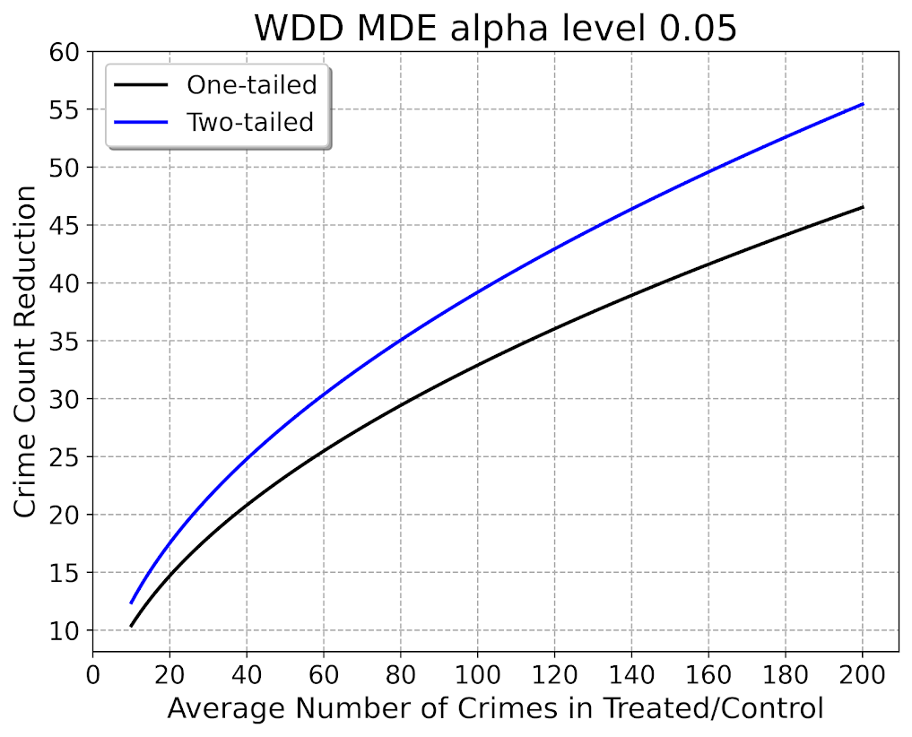
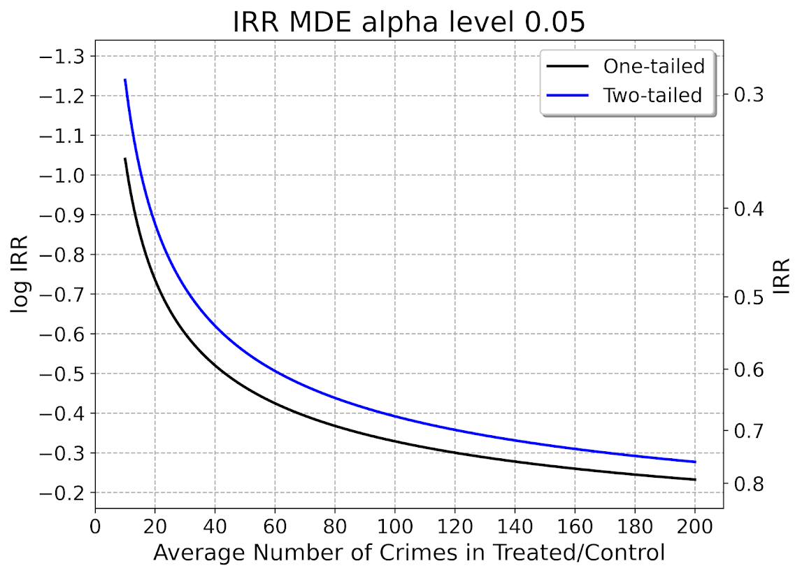
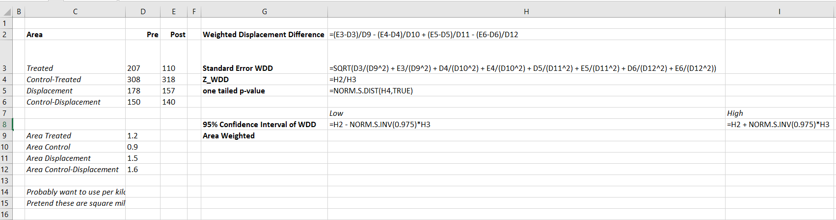
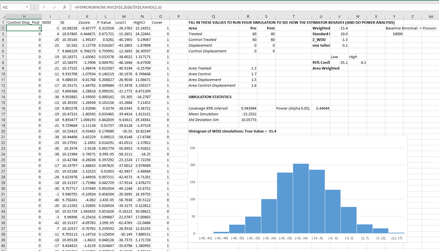
Sophie Curtis-Ham asks whether I can extend my WDD rate example to using the Poisson regression approach I outline. I spent some time and figured out the answer is yes.

First, if you install my R package ptools, we can use the same example in that blog post showing rates (or as per area, e.g. density) in my internal wdd function using R code (Wheeler & Ratcliffe, 2018):

library(ptools)

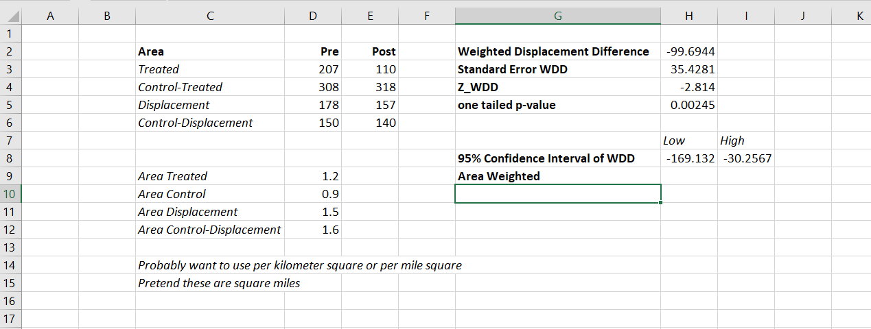
crime <- c(207,308,178,150,110,318,157,140)
type <- c('t','ct','d','cd','t','ct','d','cd')
ti <- c(0,0,0,0,1,1,1,1)
ar <- c(1.2,0.9,1.5,1.6,1.2,0.9,1.5,1.6)

df <- data.frame(crime,type,ti,ar)

# The order of my arguments is different than the 
# dataframe setup, hence the c() selections
weight_wdd <- wdd(control=crime[c(2,6)],
                  treated=crime[c(1,5)],
                  disp_control=crime[c(4,8)],
                  disp_treated=crime[c(3,7)],
                  area_weights=ar[c(2,1,4,3)])

# Estimate -91.9 (31.5) for local

So here the ar vector is a set of areas (imagine square miles or square kilometers) for treated/control/displacement/displacementcontrol areas. But it would work the same if you wanted to do person per-capita rates as well.

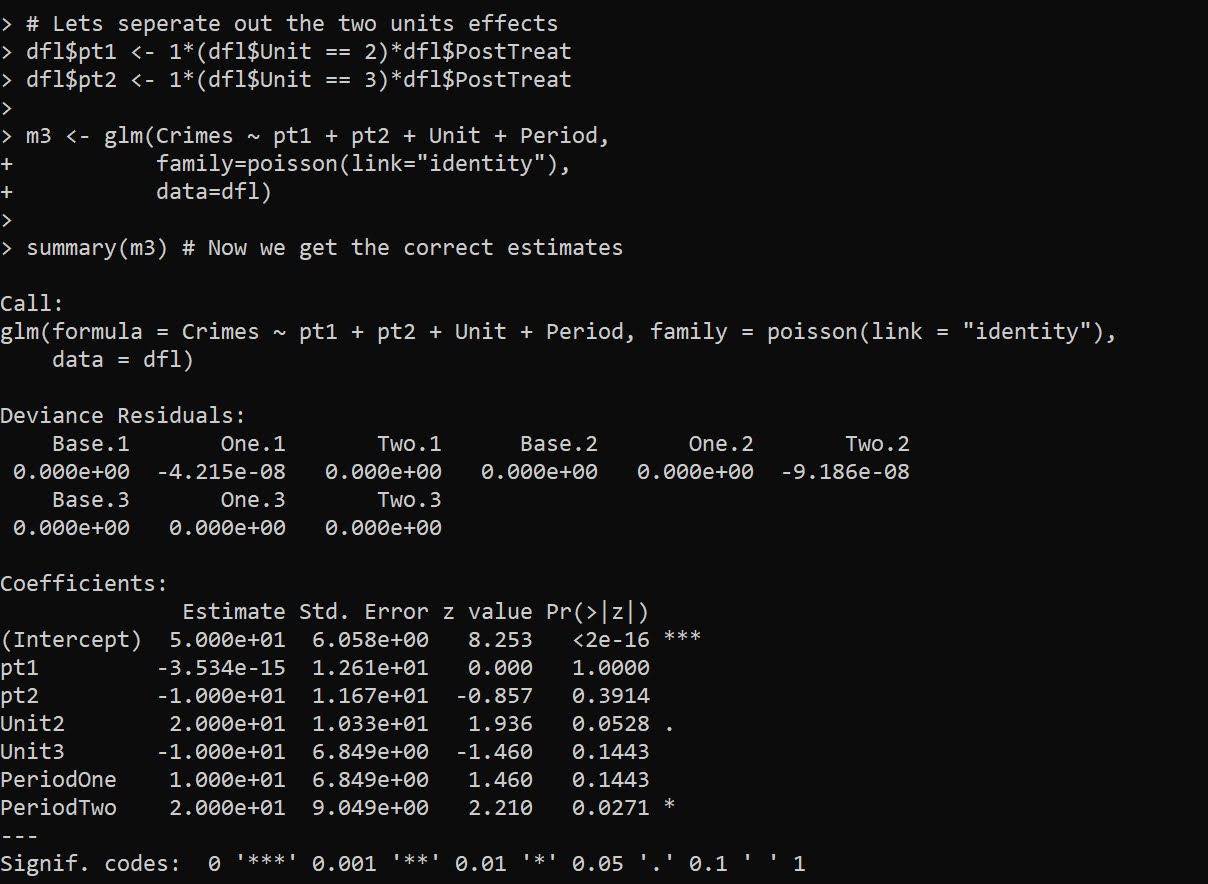
Note that the note says the estimate for the local effect, in the glm I will show I am just estimating the local, not the displacement effect. At first I tried using an offset, and that did not change the estimate at all:

# Lets do a simpler example with no displacement
df_nod <- df[c(1,2,5,6),]
df_nod['treat'] <- c(1,0,1,0)
df_nod['post'] <- df_nod['ti']

# Attempt 1, using offset
m1 <- glm(crime ~ post + treat + post*treat + offset(log(ar)),
          data=df_nod,
          family=poisson(link="identity"))
summary(m1) # estimate is  -107 (30.7), same as no weights WDD

Maybe to get the correct estimate via the offset approach you need to do some post-hoc weighting, I don’t know. But we can use weights and estimate the rate on the left hand side.

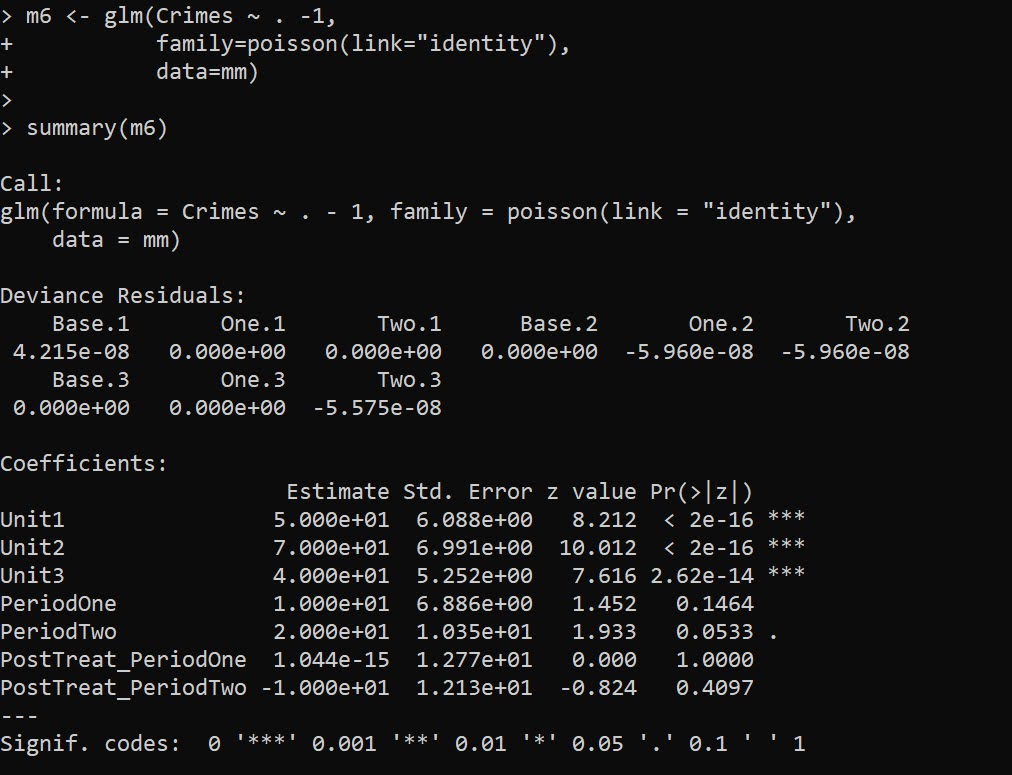
# Attempt 2, estimate rate and use weights
# suppressWarnings is for non-integer notes
df_nod['rate'] <- df_nod['crime']/df_nod['ar']
m2 <- suppressWarnings(glm(rate ~ post + treat + post*treat,
          data=df_nod,
          weights=ar,
          family=poisson(link="identity")))
summary(m2) # estimate is same as no weights WDD, -91.9 (31.5)

The motivation again for the regression approach is to extend the WDD test to scenarios more complicated than simple pre/post, and using rates (e.g. per population or per area) seems to be a pretty simple thing people may want to do!

Example 2: Clustering of Observations

Had a bit of a disagreement at work the other day – statistical models used for inference of coefficients on the right hand side often make the “IID” assumption – independent and identically distributed residuals (or independent observations conditional on the model). This is almost entirely focused on standard errors for right hand side coefficients, when using machine learning models for purely prediction it may not matter at all.

Even if interested in inference, it may be the solution is to simply weight the regression. Consider the most extreme case, we simply double count (or here repeat count observations 100 times over):

# Simulating simple Poisson model
# but replicating data
set.seed(10)
n <- 600
repn <- 100
id <- 1:n
x <- runif(n)
l <- 0.5 + 0.3*x
y <- rpois(n,l)
small_df <- data.frame(y,x,id)
big_df <- data.frame(y=rep(y,repn),x=rep(x,repn),id=rep(id,repn))

# With small data 
mpc <- glm(y ~ x, data=small_df, family=poisson)
summary(mpc)

# Note same coefficients, just SE are too small
mpa <- glm(y ~ x, data=big_df, family=poisson)

vcov(mpc)/vcov(mpa) # ~ 100 times too small

So as expected, the standard errors are 100 times too small. Again this does not cause bias in the equation (and so will not cause bias if the equation is used for predictions). But if you are making inferences for coefficients on the right hand side, this suggests you have way more precision in your estimates than you do in reality. One solution is to simply weight the observations inverse the number of repeats they have:

big_df$w <- 1/repn
mpw <- glm(y ~ x, weight=w, data=big_df, family=poisson)
summary(mpw)
vcov(mpc)/vcov(mpw) # correct covariance estimates

And this will be conservative in many circumstances, if you don’t have perfect replication across observations. Another approach though is to cluster your standard errors, which uses data to estimate the residual autocorrelation inside of your groups.

library(sandwich)
adj_mpa <- vcovCL(mpa,cluster=~id,type="HC2")
vcov(mpc)/adj_mpa   # much closer, still *slightly* too small

I use HC2 here as it uses small sample degree of freedom corrections (Long & Ervin, 2000). There are quite a few different types of cluster corrections. In my simulations HC2 tends to be the “right” choice (likely due to the degree of freedom correction), but I don’t know if that should generally be the default for clustered data, so caveat emptor.

Note again though that the cluster standard error adjustments don’t change the point estimates at all – they simply adjust the covariance matrix estimates for the coefficients on the right hand side.

Example 3: What estimate do you want?

So in the above example, I exactly repeated everyone 100 times. You may have scenarios where you have some observations repeated more times than others. So above if I had one observation repeated 10 times, and another repeated 2 times, the correct weights in that scenario would be 1/10 and 1/2 for each row inside the clusters/repeats. Here is another scenario though where we want to weight up repeat observations though – it just depends on the exact estimate you want.

A questioner wrote in with an example of a discrete choice type set up, but some respondents are repeated in the data (e.g. chose multiple responses). So imagine we have data:

Person,Choice
  1      A  
  1      B  
  1      C  
  2      A  
  3      B  
  4      B  

If you want to know the estimate in this data, “pick a random person-choice, what is the probability of choosing A/B/C?”, the answer is:

A - 2/6
B - 3/6
C - 1/6

But that may not be what you really want, it may be you want “pick a random person, what is the probability that they choose A/B/C?”, so in that scenario the correct estimate would be:

A - 2/4
B - 3/4
C - 1/4

To get this estimate, we should weight up responses! So typically each row would get a weight of 1/nrows, but here we want the weight to be 1/npersons and constant across the dataset.

Person,Choice,OriginalWeight,UpdateWeight
  1      A      1/6             1/4
  1      B      1/6             1/4
  1      C      1/6             1/4
  2      A      1/6             1/4
  3      B      1/6             1/4
  4      B      1/6             1/4

And this extends to whatever regression model if you want to model the choices as a function of additional covariates. So here technically person 1 gets triple the weight of persons 2/3/4, but that is the intended behavior if we want the estimate to be “pick a random person”.

Depending on the scenario you could do two models – one to estimate the number of choices and another to estimate the probability of a specific choice, but most people I imagine are not using such models for predictions so much as they are for inferences on the right hand side (e.g. what influences your choices).

Example 4: Cross-classified data

The last example has to do with observations that are nested within multiple hierarchical groups. One example that comes up in spatial criminology – we want to do analysis of some crime reduction/increase in a buffer around a point of interest, but multiple buffers overlap. A solution is to weight observations by the number of groups they overlap.

For example consider converting incandescent street lamps to LED (Kaplan & Chalfin, 2021). Imagine that we have four street lamps, {c1,c2,t1,t2}. The figure below display these four street lamps; the t street lamps are treated, and the c street lamps are controls. Red plus symbols denote crime locations, and each street lamp has a buffer of 1000 feet. The two not treated circle street lamps overlap, and subsequently a simple buffer would double-count crimes that fall within both of their boundaries.

If one estimated a treatment effect based on these buffer counts, with the naive count within buffer approach, one would have:

c1 = 3    t1 = 1
c2 = 4    t2 = 0

Subsequently an average control would then be 3.5, and the average treated would be 0.5. Subsequently one would have an average treatment effect of 3. This however would be an overestimate due to the overlapping buffers for the control locations. Similar to example 3 it depends on how exactly you want to define the average treatment effect – I think a reasonable definition is simply the global estimate of crimes reduced divided by the total number of treated areas.

To account for this, you can weight individual crimes. Those crimes that are assigned to multiple street lamps only get partial weight – if they overlap two street lamps, the crimes are only given a weight of 0.5, if they overlap three street lamps within a buffer area those crimes are given a weight of 1/3, etc. With such updated weighted crime estimates, one would then have:

c1 = 2    t1 = 1
c2 = 3    t2 = 0

And then one would have an average of 2.5 crimes in the control street lamps, and subsequently would have a treatment effect reduction per average street lamp of 2 crimes overall.

This idea I first saw in Snijders & Bosker (2011), in which they called this cross-classified data. I additionally used this technique with survey data in Wheeler et al. (2020), in which I nested responses in census tracts. Because responses were mapped to intersections, they technically could be inside multiple census tracts (or more specifically I did not know 100% what tract they were in). I talk about this issue in my dissertation a bit with crime data, see pages 90-92 (Wheeler, 2015). In my dissertation using D.C. data, if you aggregated that data to block groups/tracts the misallocation error is likely ~5% in the best case scenario (and depending on data and grouping, could be closer to 50%).

But again I think a reasonable solution is to weight observations, which is not much different to Hipp & Boessan’s (2013) egohoods.

References

Staggered Treatment Effect DiD count models

So I have been dealing with various staggered treatments for difference-in-difference (DiD) designs for crime data analysis on how interventions reduce crime. I’ve written about in the past mine and Jerry’s WDD estimator (Wheeler & Ratcliffe, 2018), as well as David Wilson’s ORR estimator (Wilson, 2022).

There has been quite a bit of work in econometrics recently describing how the traditional way to apply this design to staggered treatments using two-way fixed effects can be misleading, see Baker et al. (2022) for human readable overview.

The main idea is that in the scenario where you have treatment heterogeneity (TH from here on) (either over time or over units), the two-way fixed effects estimator is a weird average that can misbehave. Here are just some notes of mine though on fitting the fully saturated model, and using post-hoc contrasts (in R) to look at that TH as well as to estimate more reasonable average treatment effects.

So first, we can trick R to use glm to get my WDD estimator (or of course Wilson’s ORR estimator) for the DiD effect with count data. Here is a simple example from my prior blog post:

# R code for DiD model of count data
count <- c(50,30,60,55)
post <- c(0,1,0,1)
treat <- c(1,1,0,0)

df <- data.frame(count,post,treat)

# Wilson ORR estimate
m1 <- glm(count ~ post + treat + post*treat,data=df,family="poisson")
summary(m1)

And here is the WDD estimate using glm passing in family=poisson(link="identity"):

m2 <- glm(count ~ post + treat + post*treat,data=df,
          family=poisson(link="identity"))
summary(m2)

And we can see this is the same as my WDD in the ptools package:

library(ptools) # via https://github.com/apwheele/ptools
wdd(c(60,55),c(50,30))

Using glm will be more convenient than me scrubbing up all the correct weights, as I’ve done in the past examples (such as temporal weights and different area sizes). It is probably the case you can use different offsets in regression to accomplish similar things, but for this post just focusing on extending the WDD to varying treatment timing.

Varying Treatment Effects

So the above scenario is a simple pre/post with only one treated unit. But imagine we have two treated units and three time periods. This is very common in real life data where you roll out some intervention to more and more areas over time.

So imagine we have a set of crime data, G1 is rolled out first, so the treatment is turned on for periods One & Two, G2 is rolled out later, and so the treatment is only turned on for period Two.

Period    Control     G1     G2
Base          50      70     40
One           60      70     50
Two           70      80     50

I have intentionally created this example so the average treatment effect per period per unit is 10 crimes. So no TH. Here is the R code to show off the typical default two-way fixed effects model, where we just have a dummy variable for unit+timeperiods that are treated.

# Examples with Staggered Treatments
df <- read.table(header=TRUE,text = "
 Period    Control     G1     G2
 Base          50      70     40
 One           60      70     50
 Two           70      80     50
")

# reshape wide to long
nvars <- c("Control","G1","G2")
dfl <- reshape(df,direction="long",
               idvar="Period",
               varying=list(nvars),
               timevar="Unit")

dfl$Unit <- as.factor(dfl$Unit)
names(dfl)[3] <- 'Crimes'

# How to set up design matrix appropriately?
dfl$PostTreat <- c(0,0,0,0,1,1,0,0,1)

m1 <- glm(Crimes ~ PostTreat + Unit + Period,
          family=poisson(link="identity"),
          data=dfl)

summary(m1) # TWFE, correct point estimate

The PostTreat variable is the one we are interested in, and we can see that we have the correct -10 estimate as we expected.

OK, so lets create some treatment heterogeneity, here now G1 has no effects, and only G2 treatment works.

dfl[dfl$Unit == 2,'Crimes'] <- c(70,80,90)

m2 <- glm(Crimes ~ PostTreat + Unit + Period,
          family=poisson(link="identity"),
          data=dfl)

summary(m2) # TWFE, estimate -5.29, what?

So you may naively think that this should be something like -5 (average effect of G1 + G2), or -3.33 (G1 gets a higher weight since it is turned on for the 2 periods, whereas G2 is only turned on for 1). But nope rope, we get -5.529.

We can estimate the effects of G1 and G2 seperately though in the regression equation:

# Lets seperate out the two units effects
dfl$pt1 <- 1*(dfl$Unit == 2)*dfl$PostTreat
dfl$pt2 <- 1*(dfl$Unit == 3)*dfl$PostTreat

m3 <- glm(Crimes ~ pt1 + pt2 + Unit + Period,
          family=poisson(link="identity"),
          data=dfl)

summary(m3) # Now we get the correct estimates

And now we can see that as expected, the effect for G2 is the pt2 coefficient, which is -10. And the effect for G1, the pt1 coefficient, is only floating point error different than 0.

To then get a cumulative crime reduction effect for all of the areas, we can use the multcomp library and the glht function and construct the correct contrast matrix. Here the G1 effect gets turned on for 2 periods, and the G2 effect is only turned on for 1 period.

library(multcomp)
cont <- matrix(c(0,2,1,0,0,0,0),1)
cumtreat <- glht(m3,cont) # correct cumulative
summary(cumtreat)

And if we want an ‘average treatment effect per unit and per period’, we just change the weights in the contrast matrix:

atreat <- glht(m3,cont/3) # correct average over 3 periods
summary(atreat)

And this gets us our -3.33 that is a more reasonable average treatment effect. Although you would almost surely just focus on that the G2 area intervention worked and the G1 area did not.

You can also fit this model alittle bit easier using R’s style formula instead of rolling your own dummy variables via the formula Crimes ~ PostTreat:Unit + Unit + Period:

But, glht does not like it when you have dropped levels in these interactions, so I don’t do this approach directly later on, but construct the model matrix and drop non-varying columns.

Next lets redo the data again, and now have time varying treatments. Now only period 2 is effective, but it is effective across both the G1 and G2 locations. Here is how I construct the model matrix, and what the resulting sets of dummy variables looks like:

# Time Varying Effects
# only period 2 has an effect

dfl[dfl$Unit == 2,'Crimes'] <- c(70,80,80)

# Some bookkeeping to make the correct model matrix
mm <- as.data.frame(model.matrix(~ -1 + PostTreat:Period + Unit + Period, dfl))
mm <- mm[,names(mm)[colSums(mm) > 0]] # dropping zero columns
names(mm) <- gsub(":","_",names(mm))  # replacing colon
mm$Crimes <- dfl$Crimes
print(mm)

Now we can go ahead and fit the model without the intercept.

# Now can fit the model
m6 <- glm(Crimes ~ . -1,
          family=poisson(link="identity"),
          data=mm)

summary(m6)

And you can see we estimate the correct effects here, PostTreat_PeriodOne has a zero estimate, and PostTreat_PeriodTwo has a -10 estimate. And now our cumulative crimes reduced estimate -20

cumtreat2 <- glht(m6,"1*PostTreat_PeriodOne + 2*PostTreat_PeriodTwo=0")
summary(cumtreat2)

And if we did the average, it would be -6.66.

Now for the finale – we can estimate the saturated model with time-and-unit varying treatment effects. Here is what the design matrix looks like, just a bunch of columns with a single 1 turned on:

# Now for the whole shebang, unit and period effects
mm2 <- as.data.frame(model.matrix(~ -1 + Unit:PostTreat:Period + Unit + Period, dfl))
mm2 <- mm2[,names(mm2)[colSums(mm2) > 0]] # dropping zero columns
names(mm2) <- gsub(":","_",names(mm2))  # replacing colon
mm2$Crimes <- dfl$Crimes
print(mm2)

And then we can fit the model the same way:

m7 <- glm(Crimes ~ . -1,
          family=poisson(link="identity"),
          data=mm2)

summary(m7) # Now we get the correct estimates

And you can see our -10 estimate for Unit2_PostTreat_PeriodTwo and Unit3_PostTreat_PeriodTwo as expected. You can probably figure out how to get the cumulative or the average treatment effects at this point:

tstr <- "Unit2_PostTreat_PeriodOne + Unit2_PostTreat_PeriodTwo + Unit3_PostTreat_PeriodTwo = 0"
cumtreat3 <- glht(m7,tstr)
summary(cumtreat3)

We can also use this same framework to get a unit and time varying estimate for Wilson’s ORR estimator, just using family=poisson with its default log link function:

m8 <- glm(Crimes ~ . -1,
          family=poisson,
          data=mm2)

summary(m8)

It probably does not make sense to do a cumulative treatment effect in this framework, but I think an average is OK:

avtreatorr <- glht(m8,
  "1/3*Unit2_PostTreat_PeriodOne + 1/3*Unit2_PostTreat_PeriodTwo + 1/3*Unit3_PostTreat_PeriodTwo = 0")
summary(avtreatorr)

So the average linear coefficient is -0.1386, and if we exponentiate that we have an IRR of 0.87, so on average when a treatment occurred in this data a 13% reduction. (But beware, I intentionally created this data so the parallel trends for the DiD analysis were linear, not logarithmic).

Note if you are wondering about robust estimators, Wilson suggests using quasipoisson, e.g. glm(Crimes ~ . -1,family="quasipoisson",data=mm2), which works just fine for this data. The quasipoisson or other robust estimators though return 0 standard errors for the saturated family=poisson(link="identity") or family=quasipoisson(link="identity").

E.g. doing

library(sandwich)
cumtreat_rob <- glht(m7,tstr,vcov=vcovHC,type="HC0")
summary(cumtreat_rob)

Or just looking at robust coefficients in general:

library(lmtest)
coeftest(m7,vcov=vcovHC,type="HC0")

Returns 0 standard errors. I am thinking with the saturated model and my WDD estimate, you get the issue with robust standard errors described in Mostly Harmless Econometrics (Angrist & Pischke, 2008), that they misbehave in small samples. So I am a bit hesitant to suggest them without more work to establish they behave the way they should in smaller samples.

References

  • Angrist, J.D., & Pischke, J.S. (2008). Mostly Harmless Econometrics. Princeton University Press.
  • Baker, A.C., Larcker, D.F., & Wang, C.C. (2022). How much should we trust staggered difference-in-differences estimates? Journal of Financial Economics, 144(2), 370-395.
  • Wheeler, A.P., & Ratcliffe, J.H. (2018). A simple weighted displacement difference test to evaluate place based crime interventions. Crime Science, 7(1), 1-9.
  • Wilson, D.B. (2022). The relative incident rate ratio effect size for count-based impact evaluations: When an odds ratio is not an odds ratio. Journal of Quantitative Criminology, 38(2), 323-341.

Minimum detectable effect sizes for place based designs

So I was reading Blattman et al.’s (2018) work on a hot spot intervention in Bogotá the other day. It is an excellent piece, but in a supplement to the paper Blattman makes the point that while his study is very high powered to detect spillovers, most other studies are not. I am going to detail here why I disagree with his assessment on that front.

In appendix A he has two figures, one for the direct effect comparing the historical hot spot policing studies (technically he uses the older 2014 Braga study, but here is the cite for the update Braga et al., 2020).

The line signifies a Cohen’s D of 0.17, and here is the same graph for the spillover estimates:

So you can see Blattman’s study in total number of spatial units of analysis breaks the chart so to speak. You can see however there are plenty of hot spot studies in either chart that reported statistically significant differences, but do not meet the 0.17 threshold in Chris’s chart. How can this be? Well, Chris is goal switching a bit here, he is saying using his estimator the studies appear underpowered. The original studies on the graph though did not necessarily use his particular estimator.

The best but not quite perfect analogy I can think of is this. Imagine I build a car that gets better gas mileage compared to the current car in production. Then someone critiques this as saying the materials that go into production of the car have worse carbon footprints, so my car is actually worse for the environment. It would be fine to argue a different estimate of total carbon footprint is reasonable (here Chris could argue his estimator is better than the ones the originally papers used). It is wrong though to say you don’t actually improve gas mileage. So it is wrong for Chris to say the original articles are underpowered using his estimator, they may be well powered using a different estimator.

Indeed, using either my WDD estimator (Wheeler & Ratcliffe, 2018) or Wilson’s log IRR estimator (Wilson, 2021), I will show how power does not grow with more experimental units, but with a larger baseline number of crimes for those estimators. They both only have two spatial units of analysis, so in Chris’s chart will never gain more power.

One way I think about the issue for spatial designs is this – you could always split up a spatial lattice into ever finer and finer spatial units of analysis. For example Chris could change his original design to use addresses instead of street segments, and split up the spillover buffers into finer slices as well. Do you gain something for doing nothing though? I doubt it.

I describe in my dissertation how finer spatial units of analysis allow you to check for finer levels of spatial spillovers, e.g. can check if crime spills over from the back porch to the front stoop (Wheeler, 2015). But when you do finer spatial units, you get more cold floor effects as well due to the limited nature of crime counts – they cannot go below 0. So designs with lower baseline crime rates tend to show lower power (Hinkle et al., 2013).

MDE for the WDD and log IRR

For minimum detectable effect (MDE) sizes for OLS type estimators, you need to specify the variance you expect the underlying treated/control groups to have. With the count type estimators I will show here, the variance is fixed according to the count. So all I need to specify is the alpha level of the test. Here I will do a default of 0.05 alpha level (with different lines for one-tailed vs two-tailed). The other assumption is the distribution of crime counts between treated/control areas. Here I assume they are all equal, so 4 units (pre/post and treated/control). For my WDD estimator this actually does not matter, for the later IRR estimator though it does (so the lines won’t really be exact for his scenario).

So here is the MDE for mine and Jerry’s WDD estimator:

What this means is that if you have an average of 20 crimes in the treated/control areas for each time period separately, you would need to find a reduction of 15 crimes to meet this threshold MDE for a one-tailed. It is pretty hard when starting with low baselines! For an example close to this, if the treated area went from 24 to 9, and the control area was 24 to 24, this would meet the minimal treated reduction of 15 crimes in this example.

And here is the MDE for the log IRR estimator. The left hand Y axis has the logged effect, and the right hand side has the exponentiated IRR (incident rate ratio).

Since the IRR is commonly thought of as a percent reduction, this suggests even with baselines of 200 crimes, for Wilson’s IRR estimator you need percent reductions of over 20% relative to control areas.

So I have not gone through the more recent Braga et al. (2020) meta-analysis. I do not know if they have the data readily available to draw the points on this plot the same as in the Blattman article. To be clear, it may be Blattman is right and these studies are underpowered using either his or my estimator, I am not sure. (I think they probably are quite underpowered to detect spillover, since this presumably will be an even smaller amount than the direct effect. But that would not explain estimates of diffusion of benefits commonly found in these studies!)

I also do not know if one estimator is clearly better or not – for example Blattman could use my estimator if he simply pools all treated/control areas. This is not obviously better than his approach though, and foregoes any potential estimates of treatment effect variance (I will be damned if I can spell that word starting with het even close enough for autocorrect). But maybe the pooled estimate is OK, Blattman does note that he has cold floor effects in his linear estimator – places with higher baselines have larger effects. This suggests Wilson’s log IRR estimator with the pooled data may be just fine and dandy for example.

Python code

Here is the python code in its entirety to generate the above two graphs. You can see the two functions to calculate the MDE given an alpha level and average crime counts in each area if you are planning your own study, the wdd_mde and lirr_mde functions.

'''
Estimating minimum detectable effect sizes
for place based crime interventions

Andy Wheeler
'''

import numpy as np
from scipy.stats import norm
import matplotlib
import matplotlib.pyplot as plt
import os
my_dir = r'D:\Dropbox\Dropbox\Documents\BLOG\min_det_effect'
os.chdir(my_dir)

#########################################################
#Settings for matplotlib

andy_theme = {'axes.grid': True,
              'grid.linestyle': '--',
              'legend.framealpha': 1,
              'legend.facecolor': 'white',
              'legend.shadow': True,
              'legend.fontsize': 14,
              'legend.title_fontsize': 16,
              'xtick.labelsize': 14,
              'ytick.labelsize': 14,
              'axes.labelsize': 16,
              'axes.titlesize': 20,
              'figure.dpi': 100}

matplotlib.rcParams.update(andy_theme)
#########################################################

#########################################################
# Functions for MDE for WDD and logIRR estimator


def wdd_mde(avg_counts,alpha=0.05,tails='two'):
    se = np.sqrt( avg_counts*4 )
    if tails == 'two':
        a = 1 - alpha/2
    elif tails == 'one':
        a = 1 - alpha
    z = norm.ppf(a)
    est = z*se
    return est

def lirr_mde(avg_counts,alpha=0.05,tails='two'):
    se = np.sqrt( (1/avg_counts)*4 )
    if tails == 'two':
        a = 1 - alpha/2
    elif tails == 'one':
        a = 1 - alpha
    z = norm.ppf(a)
    est = z*se
    return est

# Generating regular grid from 10 to 200
cnts = np.arange(10,201)
wmde1 = wdd_mde(cnts, tails='one')
wmde2 = wdd_mde(cnts)

imde1 = lirr_mde(cnts, tails='one')
imde2 = lirr_mde(cnts)

# Plot for WDD MDE
fig, ax = plt.subplots(figsize=(8,6))
ax.plot(cnts, wmde1,color='k',linewidth=2, label='One-tailed')
ax.plot(cnts, wmde2,color='blue',linewidth=2, label='Two-tailed')
ax.set_axisbelow(True)
ax.set_xlabel('Average Number of Crimes in Treated/Control')
ax.set_ylabel('Crime Count Reduction')
ax.legend(loc='upper left')
plt.xticks(np.arange(0,201,20))
plt.yticks(np.arange(10,61,5))
plt.title("WDD MDE alpha level 0.05")
plt.savefig('WDD_MDE.png', dpi=500, bbox_inches='tight')

# Plot for IRR MDE
fig, ax = plt.subplots(figsize=(8,6))
ax2 = ax.secondary_yaxis("right", functions=(np.exp, np.log))
ax.plot(cnts,-1*imde1,color='k',linewidth=2, label='One-tailed')
ax.plot(cnts,-1*imde2,color='blue',linewidth=2, label='Two-tailed')
ax.set_axisbelow(True)
ax.set_xlabel('Average Number of Crimes in Treated/Control')
ax.set_ylabel('log IRR')
ax.set_ylim(-0.16, -1.34)
ax.legend(loc='upper right')
ax.set_yticks(-1*np.arange(0.2,1.31,0.1))
ax2.set_ylabel('IRR')
ax2.grid(False)
plt.xticks(np.arange(0,201,20))
plt.title("IRR MDE alpha level 0.05")
plt.savefig('IRR_MDE.png', dpi=500, bbox_inches='tight')

#########################################################

References

Comparing the WDD vs the Wilson log IRR estimator

So this is maybe my final post on the WDD estimator for the time being (Wheeler & Ratcliffe, 2018). Recently David Wilson had an article in JQC that proposes a different estimator using the same basic information, just pre-post crime counts for treated and control areas (Wilson, 2021). So say we had the table:

         Pre   Post
Treated   50     30
Control   60     55

So in this scenario, my WDD estimate is -20 in the treated area, and -5 in the control area, so the overall estimate is -20 – -5 = -15.

30 - 50 - (55 - 60) = -15

So an estimated reduction of -15 crimes overall. David’s estimator is the logged incident rate ratio (IRR), and so is just like above, except logs all of the values:

log(30) - log(50) - ( log(55) - log(60) ) = -0.4238142

This is a logged incident rate adjustment, so most of the time people exponentiate this value, which is exp(-0.4238142) = 0.6545455. So this suggests crime is reduced by approximately 35% in the treated area relative to the control area in this hypothetical. Or another way to write it is (30/50)/(55/60) = 0.6545455.

So instead of a linear estimate of the total numbers of crimes reduced, this is an estimate of the overall rate reduction. So this begs the question when would you prefer my WDD vs the IRR? I will try to answer that below – in short I think David’s estimator makes sense for meta-analyses (as I have said before in reference to the work in Braga & Weisburd, 2020). But for an individual agency doing an experimental evaluation I much prefer my estimator. The skinny of this logic is that we only really care about the overall crime reduction estimate from a cost-benefit analysis perspective. Backing out this total crime reduction count estimate from David’s IRR estimate can result in some funny business for an individual study.

Identifying Assumptions

So there are really two different assumptions my WDD estimator and David’s IRR estimator make. To generate a standard error estimate around the point estimate for either estimator, both require the data are Poisson distributed. So that makes no difference between the two. The assumption that really distinguishes between the WDD and the IRR estimate is the parallel trends assumption. The WDD assumes parallel trends are on the linear scale, whereas the IRR assumes parallel trends are on the ratio scale.

What exactly does this mean? Imagine we have a treated and control area, but look at the crime trends per time period before the treatment occurred. This set of areas has a set of parallel trends on the linear scale:

Time Treated Control
 0     50      60
 1     40      50
 2     45      55
 3     50      60

When the treated area goes down by 10 crimes, the control area goes down by 10 crimes. That is a parallel on the linear scale. Whereas this scenario is parallel on the ratio scale:

Time Treated Control
 0     50      60
 1     40      48
 2     45      54
 3     50      60

When crime goes down by 20% in the treated area, it goes down by 20% in the control area.

So while this gives a potential way to say you should use the WDD (parallel on the linear scale), or the IRR (parallel on the ratio scale), in practice it is not so simple. For one thing, if you only has the pre/post counts of crime, you cannot distinguish between these two scenarios. You can only tell in the case you have historical data to examine.

For a second part of this, you typically can choose your own control area (see for example the synthetic control estimator). So in most scenarios you could choose a control area to obey the linear or the ratio parallel trends assumption if you wanted to. However it may be in many scenarios there is a natural/easy control area, and you may see what is a better fit in that case for linear/ratio.

A final wee bit of a perverse aspect about this I will mention – pretend we have a treated/control area have approximately the same baseline crime counts/rates:

Time Treated Control
 0      30     30
 1      25     25
 2      20     20
 3      25     25

You actually cannot tell in this scenario whether the parallel trends are on the linear scale for my WDD or the ratio scale for the IRR estimate. They are consistent with either! In practice I think in many cases it will be like this – with noisy data, if you choose a control area that has approximately the same baseline crime counts, it will be quite hard to tell whether the linear parallel trends makes more sense or the ratio parallel trends makes more sense.

There are situations where the linear changes do not make sense, but they tend to be scenarios such as the control area has very little crime (so cannot go below 0 to match larger ups/downs in the treated area). So in that case sure the IRR is plausible and the WDD is not, but those are cases where the control area itself is quite questionable. Also note the IRR is not defined for any cells with 0 crimes – but again it is not good for either of our estimators in that case (although mine won’t fail to spit out a number, the power is so low the number it spits out won’t be worth much).

Bias/Coverage

So I have adapted the same simulation code I used in prior studies/blog posts to evaluate the null distribution and the coverage of David’s IRR estimator. I partly did not pursue it initially back when me and Jerry were discussing this idea, because I thought it would be biased. Generalized linear models are based on maximum likelihood estimators, which are only asymptotically valid. In short it appears I was wrong here and David’s IRR estimator is fine even with just four observations, at least for the handful of scenarios I have tried it (have not looked at very tiny counts of crime, it is undefined if any cell has 0 crimes, as you cannot take the log of 0).

Python code pasted at the very end of the blog post, but for example if we generate a set of null no changes pre/post with a baseline of 50 crimes, the logged irr estimate (converted into a z-score here) is just fine and dandy and has a very close to standard normal distribution based on 10k simulations.

So lets look at the scenario where the control area doesn’t change, but the treated area goes from 50 to 30. We can see again the point estimate in this scenario is spot on the money.

And then we can see the coverage of the logged irr estimator is spot on as well:

So if you are interested in slightly different baseline scenarios, you can use that same simulation code to check out the behavior of David’s estimator and conduct simulated power analysis the same way I have shown for the WDD estimator in prior blog posts.

So if both are unbiased and have good coverage again, why would you prefer the WDD estimator over the IRR estimator (or vice-versa)? Well, lets take the 35% reduction I talked about at the beginning of the post, and the department needs to spend $250k on extra officers to conduct whatever hot spot policing intervention. A 35% reduction may be worth it if we start with a baseline of 200 crimes (so would expect to go down to 130, for a reduction of 70 crimes). If the baseline is 20 crimes, it goes down to 13 crimes (so only a reduction of 7 crimes). The actual benefit of the IRR estimate is entirely dependent on the baseline count of crimes it is applied to.

Even if the IRR estimate is itself unbiased and has proper coverage, for even an individual study backing out the estimated reduction in total crimes from the IRR is biased. So here in this same simulated data (50 to 30 in treated, and 50 to 50 in control areas). The true count reduction is -20, and here is the point estimate on the X axis and the length of the confidence interval for each simulation on the Y axis for my WDD test. You can see they are nicely centered on -20, and the length of the confidence intervals has a very tiny variance – they are mostly just a smidge over 50 in total length. So that is probably tough to wrap your head around, but the variance of the variance estimates for the WDD are small.

Now lets do the same graph for the IRR estimate, but translated back out to a count crime reduction based on the simulated values:

We either have a ton of bias in this estimate (if the estimate of the count reduction is too large, the confidence interval is too small). Or the opposite, the estimate of the count reduction is too small, and the confidence interval is crazy wide. In Andrew Gelman’s terminology, it can result in pretty large type M (magnitude) errors in this simulated example (Gelman & Carlin, 2014). So the variance of the variance estimates in this scenario are quite large.

To be clear – if you are interested in estimating a percent reduction, by all means use David’s IRR estimator. If you however want to translate that percent reduction into an estimate of the total crimes reduced though you should use my WDD estimator in that case. You should not back out a total crimes reduced estimate from the IRR.

Final Thoughts

So I have said a few times I think the IRR estimator makes more sense for meta-analyses. Why do I think that? Well, imagine we have an underlying causal process through which a hot spots policing experiment can randomly deter/prevent a particular proportion of crimes. That underlying causal process suggests an IRR effect. And also the problem I mention with translating back to crime counts I believe should get smaller with tighter estimates.

For a causal process that is more akin to my WDD estimator, imagine some crimes will always be deterred/prevented from a hot spots policing experiment, and some will never be. And we don’t know up-front which is which, so the observed reduction is based on whatever mixture of the two we have at that particular location.

The proportion reduction seems to make more sense to me for active patrol type interventions (which are ephemeral) vs permanent CPTED like interventions which should prevent certain criminal acts in perpetuity. But of course any situation in the real world could have both occurring at the same time.

When you go and look at the meta-analysis of hot spots policing, those interventions are all over the place (Hinkle et al., 2020). I think my WDD estimate would not make sense to mash up into a final meta-analytic estimate. The IRR may not make sense either in the end, but it is plausibly more relevant to compare the IRRs from a study with a baseline of 200 crimes vs one with 40 crimes at baseline. I am not sure it makes sense to compare WDDs in that scenario. But that being said, a few of my blog posts have discussed the WDD normalized per unit area or per unit time. Those normalized estimates are probably more apples to apples in the 200 vs 40 scenario.

A final note I have not discussed here is that David discusses a correction for overdispersion, so that is a potential feather in the cap for his estimator vs the WDD. I’d be a bit hesitant though with that – only four observations to estimate the dispersion term is slicing it a bit thin IMO. But I was wrong about the original estimator, so I may be wrong about that as well. It will take simulation evidence to determine that though – David’s paper just provides the correction term, he doesn’t provide evidence for its utility with small sample data.

And to be fair I have not done simulations to see how my estimator behaves in the presence of overdispersion either. I believe it will simply just cause the standard errors to be too small, so like in Wheeler (2016), I imagine it will just require upping the interval (e.g. use a z-score of 3 instead of 2) to get proper coverage for real crime data.

References

Other Posts of Interest

Python simulation code

Here is a copy-pasted chunk of the entire python simulation code.

'''
Comparing WDD to log(IRR) from Wilson's
recent paper, https://link.springer.com/article/10.1007/s10940-021-09494-w

Andy Wheeler
'''

import pandas as pd
import numpy as np
from scipy.stats import norm
from scipy.stats import poisson
from scipy.stats import uniform
import matplotlib
import matplotlib.pyplot as plt
import os
my_dir = r'D:\Dropbox\Dropbox\Documents\BLOG\wdd_vs_irr'
os.chdir(my_dir)

#########################################################
#Settings for matplotlib

andy_theme = {'axes.grid': True,
              'grid.linestyle': '--',
              'legend.framealpha': 1,
              'legend.facecolor': 'white',
              'legend.shadow': True,
              'legend.fontsize': 14,
              'legend.title_fontsize': 16,
              'xtick.labelsize': 14,
              'ytick.labelsize': 14,
              'axes.labelsize': 16,
              'axes.titlesize': 20,
              'figure.dpi': 100}

matplotlib.rcParams.update(andy_theme)
#########################################################


#This works for the scipy functions as well
np.random.seed(seed=10)

# A function to generate the WDD estimate for simulated data
def wdd_sim(treat0,treat1,cont0,cont1,pre,post):
    tr_cr_0 = poisson.rvs(mu = treat0, size=int(pre)).sum()
    co_cr_0 = poisson.rvs(mu = cont0, size=int(pre)).sum()
    tr_cr_1 = poisson.rvs(mu = treat1, size=int(post)).sum()
    co_cr_1 = poisson.rvs(mu = cont1, size=int(post)).sum()
    # WDD estimates
    est = ( tr_cr_1/post - tr_cr_0/pre ) - ( co_cr_1/post - co_cr_0/pre )
    post2 = (1/post)**2
    pre2 = (1/pre)**2
    var_est = tr_cr_0*pre2 + tr_cr_1*post2 + co_cr_0*pre2 + co_cr_1*post2
    true_val = ( treat1 - treat0 ) - ( cont1 - cont0 )
    z_score = est / np.sqrt(var_est)
    # Wilson log IRR estimates
    true_logirr = np.log( (treat1*cont0) / (cont1*treat0) )
    est_logirr = np.log( ((tr_cr_1/post)*(co_cr_0/pre)) / ( (co_cr_1/post)*(tr_cr_0/pre) ) )
    se_logirr = np.sqrt( 1/tr_cr_1 + 1/co_cr_0 + 1/co_cr_1 + 1/tr_cr_0 )
    z_logirr = est_logirr / se_logirr
    return (tr_cr_0, co_cr_0, tr_cr_1, co_cr_0, est, var_est, true_val, z_score, true_logirr, est_logirr, se_logirr, z_logirr)

def make_data(n, treat0, treat1, cont0, cont1, pre, post):
    base = pd.DataFrame( range(n), columns=['index'])
    base['treat0'] = treat0
    if treat1 is not None:
        base['treat1'] = treat1
    else:
        base['treat1'] = base['treat0']
    if cont0 is not None:
        base['cont0'] = cont0
    else:
        base['cont0'] = base['treat0']
    if cont1 is not None:
        base['cont1'] = cont1
    else:
        base['cont1'] = base['cont0']
    base.drop(columns='index',inplace=True)
    base['pre'] = pre
    base['post'] = post
    sim_vals = base.apply(lambda x: wdd_sim(**x), axis=1, result_type='expand')
    sim_vals.columns = ['sim_t0','sim_c0','sim_t1','sim_c1','est','var_est','true_val','z_score',
                        'true_logirr','est_logirr','se_logirr','z_logirr']
    return pd.concat([base,sim_vals], axis=1)

# Coverage of the log irr estimate
# Lets look at the coverage rate for a decline from 40 to 20
def cover_logirr(data, ci=0.95):
    mult = (1 - ci)/2
    nv = norm.ppf(1 - mult)
    dif = nv*data['se_logirr']
    low = data['est_logirr'] - dif
    high = data['est_logirr'] + dif
    cover = ( data['true_logirr'] > low) & ( data['true_logirr'] < high )
    return cover

# Length of ci for WDD
def len_ci(data, ci=0.95):
    mult = (1 - ci)/2
    nv = norm.ppf(1 - mult)
    dif = nv*np.sqrt( data['var_est'] )
    low = data['est'] - dif
    high = data['est'] + dif
    return low, high, high - low

# Length of ci for IRR estimate on count scale
# This depends on the baseline estimate to multiply
# The IRR by, using the baseline average of the 
# Treatment area

def len_irr(data, ci=0.95):
    mult = (1 - ci)/2
    nv = norm.ppf(1 - mult)
    dif = nv*data['se_logirr']
    low = data['est_logirr'] - dif
    high = data['est_logirr'] + dif
    baseline = data['sim_t0']/data['pre']
    # Even if you use hypothetical, the variance is quite high
    #baseline = data['treat0']
    est_count = baseline*np.exp(data['est_logirr']) - baseline
    c1 = baseline*np.exp(low) - baseline
    c2 = baseline*np.exp(high) - baseline
    return est_count, c1, c2, np.abs(c2 - c1)

##########################
# Example with no change, lets look at the null distribution
sim_n = 10000
no_diff = make_data(sim_n, 50, 50, 50, 50, 1, 1)
no_diff['z_logirr'].describe()
##########################

##########################
# Example with equal time periods, a reduction from 50 to 30 and 50 to 50 in control area
sim_dat = make_data(sim_n, 50, 30, 50, 50, 1, 1)
sim_dat[['true_logirr','est_logirr','se_logirr']].describe()

cl = cover_logirr(sim_dat)
cl.mean()

# Compare length of CI for IRR vs WDD

# WDD length
lowdd, highwdd, lwdd = len_ci(sim_dat)
lwdd.describe()

# IRR length on the count scale
est_cnt_irr, lo_irr, hi_irr, ln_irr = len_irr(sim_dat)
ln_irr.describe()

# Scatterplot of estimated count reduction vs
# Length of CI
fig, ax = plt.subplots(figsize=(8,6))
ax.scatter(est_cnt_irr, ln_irr, c='k', 
            alpha=0.1, s=4)
ax.set_axisbelow(True)
ax.set_xlabel('Estimated Count Reduction [IRR]')
ax.set_ylabel('Length of CI on count scale [IRR]')
plt.savefig('IRR_Len_Est.png', dpi=500, bbox_inches='tight')
plt.show()

# Lets compare to the WDD estimate
fig, ax = plt.subplots(figsize=(8,6))
ax.scatter(sim_dat['est'], lwdd, c='k', 
            alpha=0.1, s=4)
ax.set_axisbelow(True)
ax.set_xlabel('Estimated Count Reduction [WDD]')
ax.set_ylabel('Length of CI on count scale [WDD]')
plt.savefig('WDD_Len_Est.png', dpi=500, bbox_inches='tight')
plt.show()
##########################

The WDD test with different area sizes

So I have two prior examples of weighting the WDD test (a simple test for pre-post crime counts in an experimental setting):

And a friend recently asked about weighting for different areas, so the test is crime reduction per area density instead of overall counts. First before I get into the example, this isn’t per se necessary. All that matters in the end for this test to be valid is 1) the crime data are Poisson distributed, 2) the control areas follow parallel trends to the treated area. So based on this I’ve advocated that it is ok to have a control area be ‘the rest of the city’ for example.

Some of my work on long term crime trends at micro places, shows low-crime and high-crime areas all tend to follow the same overall temporal trends (and Martin Andresen’s related work one would come to the same conclusion). So that would suggest you can aggregate up many low crimes to make a reasonable control comparison to a hot spot treated area.

So as I will show weighting by area is possible, but it actually changes the identification strategy slightly (whereas the prior two weighting examples do not) – the parallel trends assumption needs to be on the crime per area estimate, as opposed to the original count scale. Since the friend who asked about this is an Excel GURU (check out Grant’s very nice YouTube videos for crime analysis) I will show how to do the calculations in Excel, as well as how to do a simulation to show my estimator behaves as it should. (And the benefit of that is you can do power analysis based on the simulations.)

Example Calculations in Excel

I have posted an Excel spreadsheet to show the calculations here. But for a quick overview, I made the spreadsheet very similar to the original WDD calculation, you just need to insert your areas for the different treated/control/displacement areas.

And you can check out the formulas, again it is just weighting the estimator by the areas, and then making the appropriate transformations to the variance estimates.

I have an added extra portion of this though – a simulation tab to show the estimator works.

Only thing to note, a way to simulate to Poisson data in Excel is to generate a random number on the unit interval (0,1), and then for the distribution of interest use the inverse CDF function. There is no inverse Poisson function in Excel, but you can reasonably approximate it via the inverse binomial with a very large number of trials. I’ve tested and it is good enough for my purposes to use a base of 10k for the binomial trials.

The simulation tab on this spreadsheet you can input your own numbers for planning purposes as well. So the idea is if you think you can only reasonably reduce crimes by X amount in your targeted areas, this lets you do power analysis. So in this example, going from 60 to 40 crimes results in a power estimate of only 0.44 (so you will fail to reject the null over 5 out of 10 times, even if your intervention actually works as well as you think). But if you think you can reduce crimes from 60 to 30, the power in this example gets close to 0.8 (what you typically shoot for in up-front experiments, although there is no harm for going for higher power!). So if you have low power you may want to expand the time periods under study or expand the number of treated areas.

Wrap Up

Between this and the prior WDD examples, I have about wrapped up all the potential permutations of weighting I can think of offhand. So you can mix/match all of these different weighting strategies together (e.g. you could do multiple time periods and area weighting). It is just algebra and carrying through the correct changes to the variance estimates.

I do have one additional blog post slated in the future. David Wilson has a recent JQC article using a different estimate, but essentially the same pre/post data I am using here. The identifying assumptions are different again for this (parallel trends on the ratio scale, not the linear scale), and I will have more to say when I think you would prefer the WDD to David’s estimator. (In short I think David’s is good for meta-analysis, but I prefer my WDD for individual evaluations.)

The WDD test with different pre/post time periods

Eric Piza asked the other day if my and Jerry’s WDD test can be used when the pre/post time periods are different. The answer is yes out of the box, the identification strategy does not rely on equality of time periods. So for example, say we had two years pre and one year post data, and the crime counts in treated/control looked like this:

         Pre  Post 
Treated   80    20
Control  100    50

So then our difference-in-difference Poisson estimate of the treatment effect would be:

(20 - 80) - (50 - 100) =  -10

What the parallel trends assumption means here is that since you saw a decrease in 50 crimes in the control area, you would expect a decrease of 50 crimes in the treated area as well. The variance of this estimate is then 20 + 80 + 50 + 100 = 250, and so the standard error is sqrt(250) ~ 15.8. So this is not a statistically significant effect.

It is hard to interpret this effect size though, since it is not a standard unit of time comparison. Also the variance of the estimate will be larger if you have a longer pre time period, which is the opposite of what you want. We can actually amend the statistic though to be a per-unit-time comparison, which will reduce the variance of the estimate. It ends up being similar to my prior post on adding Harm Weights to the WDD, you can’t just pipe in the per unit time estimates in the spreadsheet I shared, but I will show here how to incorporate them into the estimator (and share some python code to show the estimator behaves as expected in simulations).

So again with a pre-time period of 2 years, and post of 1 year, we could do the prior table as per year estimates.

         Pre  Post 
Treated   40    20
Control   50    50

And here our estimate of the crime reduction effect is different:

(20 - 40) - (50 - 50) =  -20

So with a Poisson variable with a mean of 100, the variance of that variable is also 100. So here we are dividing that 100 by a constant 2 – this changes the variance to 100/(2^2). (Var(X*a) = a^2*Var(X) where X is a random variable and a is a constant.) The post variables are simply divided by one, so does not change their variance. So to carry this forward to our standard error estimate, we would calculate (edit, had some errors in this part, should be using the original counts, not the average counts, but my later python code was correct, so the simulation part is OK):

20/1 + 80/4 + 50/1 + 100/4 = 115

So you can see that our variance estimate here is much smaller, and that the standard error is sqrt(115) ~ 10.7. So here the reduction is not quite a statistically significant reduction in crimes at the 0.05 level. A 95% confidence interval would be -20 +/- 2*10.7 ~ [+1, -41]. Here the WDD estimate is easier to interpret as well, and that confidence interval corresponds to a per year estimate of somewhere between +1 and -41 crimes.

Below I share some python code to conduct simulations similar to the original WDD paper. This code will then establish the estimator has the null distribution as expected (when there are no changes it really is a standard normal distribution) and that the confidence intervals have coverage like you would expect.

Python Simulation Code

For set up, I import the libraries I need (stat distributions, numpy and pandas). I am not going to go into detail into the functions, but it allows you to generate simulated distributions in various ways to conduct analysis of the properties of my time weighted estimator I have specified above.

'''
WDD Simulation with differing time periods
Andy Wheeler
'''

import pandas as pd
import numpy as np
from scipy.stats import norm
from scipy.stats import poisson
from scipy.stats import uniform

#This works for the scipy functions
np.random.seed(seed=10)

# A function to generate the WDD estimate for simulated data
def wdd_sim(treat0,treat1,cont0,cont1,pre,post):
    tr_cr_0 = poisson.rvs(mu = treat0, size=int(pre)).sum()
    co_cr_0 = poisson.rvs(mu = cont0, size=int(pre)).sum()
    tr_cr_1 = poisson.rvs(mu = treat1, size=int(post)).sum()
    co_cr_1 = poisson.rvs(mu = cont1, size=int(post)).sum()
    est = ( tr_cr_1/post - tr_cr_0/pre ) - ( co_cr_1/post - co_cr_0/pre )
    post2 = (1/post)**2
    pre2 = (1/pre)**2
    var_est = tr_cr_0*pre2 + tr_cr_1*post2 + co_cr_0*pre2 + co_cr_1*post2
    true_val = ( treat1 - treat0 ) - ( cont1 - cont0 )
    z_score = est / np.sqrt(var_est)
    return (est, var_est, true_val, z_score)

def make_data(n, treat0, treat1, cont0, cont1, pre, post):
    base = pd.DataFrame( range(n), columns=['index'])
    base['treat0'] = treat0
    if treat1 is not None:
        base['treat1'] = treat1
    else:
        base['treat1'] = base['treat0']
    if cont0 is not None:
        base['cont0'] = cont0
    else:
        base['cont0'] = base['treat0']
    if cont1 is not None:
        base['cont1'] = cont1
    else:
        base['cont1'] = base['cont0']
    base.drop(columns='index',inplace=True)
    base['pre'] = pre
    base['post'] = post
    sim_vals = base.apply(lambda x: wdd_sim(**x), axis=1, result_type='expand')
    sim_vals.columns = ['est','var_est','true_val','z_score']
    return pd.concat([base,sim_vals], axis=1)

So for a first example, this code generates treatment/control areas with a Poisson mean of 5 in both the pre/post time periods. But, the pre time period is 4 units of time, and the post time period is only 1 unit. So this means there is no change, and the Z score estimator should on average have a 0 estimate and a standard deviation of 1. I do 10,000 simulations to keep it going a bit faster, but you can up that if you want.

# No change, with baseline of 5 crimes per unit time
sim_dat = make_data(10000, 5, 5, 5, 5, 4, 1)
sim_dat['z_score'].describe()

So here we can see these 10k simulated Poisson data have a mean z-score of 0 and a standard deviation of 1, right like we expected.

So I haven’t extensively tested, but if you have average crime counts well under 5, I would be a bit hesitant to use this estimator. (So you either need larger area aggregations or larger time aggregations.) Although you could do simulations on your own to see how it holds up.

The way I wrote the functions you can also pass in random variables as well, so here is an example with again no change, but the baseline varies uniformily from 5 to 100. And here also the pre time periods are 6, and the post time period is again just 1.

# Can pass in random functions instead of constant values
sim_n = 10000
tf = uniform.rvs(loc=5, scale=100, size=sim_n)

sim_dat2 = make_data(sim_n, tf, None, None, None, 6, 1)
sim_dat2.head()
sim_dat2['z_score'].describe()

So you can see the base simulated dataset pre/post always has the same means, but instead of being a set of constant 5’s, it changes for each row (simulation) in the dataset. And again the null distribution is right on the money with a mean of 0 and standard deviation of 1.

So those are examples of the null distribution of no changes in the time weighted estimator. This establishes that the false positive alpha rates are as you would expect. E.g. if you use the usual p-value < 0.05, if the differences are really 0 you only have a false positive reject the null 5 times out of 100.

But we also want to establish that when there is a difference, the estimator is not biased and that the variance estimates are correct. For the later part looking at the coverage rates of the confidence intervals is one way to do that. So here I show that with my hypothetical example in the intro part of this blog, the 95% and 90% confidence interval coverage rates are exactly as they should be. And the z-score estimate is right about where it should be as well.

# Lets look at the coverage rate for a decline from 40 to 20
def cover(data, ci=0.95):
    mult = (1 - ci)/2
    nv = norm.ppf(1 - mult)
    dif = nv*np.sqrt( data['var_est'] )
    low = data['est'] - dif
    high = data['est'] + dif
    cover = ( data['true_val'] > low) & ( data['true_val'] < high )
    return cover

sim_dat3 = make_data(sim_n, 40, 20, 50, 50, 2, 1)
sim_dat3.head()

# This should be centered on 2
sim_dat3['z_score'].describe()

# Should be ~ 0.9
co_90 = cover(sim_dat3, ci=0.9)
co_90.mean()

# Should be ~ 0.95
co_95 = cover(sim_dat3, ci=0.95)
co_95.mean()

So you can see the coverage is right on the money. The estimator is slightly biased downward in this simulation (should get a z-score on average around -2, but here the mean is -1.85). But it is good enough IMO to not worry about much in this situation.

Again, the original estimator without weighted for time is fine, if we do the same motions without doing weighting for different time periods, the coverage is still all fine and dandy.

# Note you can do the same coverage estimate without time weighted
sim_dat4 = make_data(sim_n, 80, 20, 100, 50, 1, 1)
sim_dat4.head()

# This should be around -0.6
sim_dat4['z_score'].describe()

co_90w = cover(sim_dat4, ci=0.9)
co_90w.mean()

co_95w = cover(sim_dat4, ci=0.95)
co_95w.mean()

So you can see again coverage is right on the money, and the z-score estimator actually has less bias than the time weighted one, it is right on the money as expected.

So why would you prefer the time weighted estimator if it shows more bias? It is because it has a lower variance, this code shows the length of the confidence intervals in the simulations.

# Does it make a difference?
def len_ci(data, ci=0.95):
    mult = (1 - ci)/2
    nv = norm.ppf(1 - mult)
    dif = nv*np.sqrt( data['var_est'] )
    low = data['est'] - dif
    high = data['est'] + dif
    return high - low

len4 = len_ci(sim_dat4)
len4.describe()

len3 = len_ci(sim_dat3)
len3.describe()

So you can see here that the non-time weighted estimator tends to have a confidence interval with a length of 62, whereas the time weighted estimator has a confidence interval on average of 42.

So above establishes that the time weighted estimator behaves as you would expect. You can also use this code to conduct some potential power analyses. So for the time weighted estimator we show, even though the reduction is around 50% in the treated area (going from 40 to 20), the power is not great, around 60%.

# Example power analyses, ONE TAILED
def reject_rate(data, alpha=0.05):
    p_vals = norm.cdf(data['z_score'])
    return p_vals < alpha
    
r3 = reject_rate(sim_dat3)
r3.mean()

So this means if you did this experiment in real life and it was that effective, you would still fail to reject the null of no differences 2/5 times.

But what if we say we will get more historical data? So 4 years back instead of just 2? How does that impact our power estimates?

# How about with more historical data
sim_dat5 = make_data(sim_n, 40, 20, 50, 50, 4, 1)
r5 = reject_rate(sim_dat5)
r5.mean()

The power goes up by alittle, to 0.67. The same is true if we up the post period to 4 time periods instead of 1:

# How about with more post data
sim_dat6 = make_data(sim_n, 40, 20, 50, 50, 4, 4)
r6 = reject_rate(sim_dat6)
r6.mean()

So now in this example you have an over 90% power to detect a crime reduction, going from 40 to 20 per time period (where the control has an average of 50 crimes per time period), if you have 4 pre time periods and 4 post time periods.

Future Stuff

So a few caveats with this. For one, you may think that since dividing per time period reduces the variance, why not divide by smaller time slivers. So instead of one year, why not divide by 365 days?

I have not studied extensively this property of the estimator. So I cannot say how it behaves with more/less time aggregation into smaller Poisson estimates. You will need to take that on yourself if you want to examine very fine time units and very small Poisson counts per unit time. Again I think a baseline rule of thumb that they should not be lower the 5 counts per unit time is the best advice I can give without doing simulations for your exact circumstances.

A second part is that with longer time periods comes the risk that the control areas are not as good. This is a problem intrinsic to synthetic control analysis as well (that I don’t believe anyone has a particular answer to). And I don’t have an answer either.

For the pre-time period, you can check the parallel trends assumption by simply plotting the two time series, they should be close to in step with one another. So that is not a big deal. But with the post time period, I think if you monitor long enough they will eventually depart from one another.

So I think it is best to set up a time period at the start you have committed to doing the experiment. And you can use the power analysis simulations like I showed to help you figure out that period. But it may be possible to extend this WDD estimate to continuously monitor an intervention (see here for example).

Amending the WDD test to incorporate Harm Weights

So I received a question the other day about amending my and Jerry Ratcliffe’s Weighted Displacement Difference (WDD) test to incorporate crime harms (Wheeler & Ratcliffe, 2018). This is a great idea, but unfortunately it takes a small bit of extra work compared to the original (from the analysts perspective). I cannot make it as simple as just piping in the pre-post crime weights into that previous spreadsheet I shared. The reason is a reduction of 10 crimes with a weight of 10 has a different variance than a reduction of 25 crimes with a weight of 4, even though both have the same total crime harm reduction (10*10 = 4*25).

I will walk through some simple spreadsheet calculations though (in Excel) so you can roll this on your own. HERE IS THE SPREADSHEET TO DOWNLOAD TO FOLLOW ALONG. What you need to do is to calculate the traditional WDD for each individual crime type in your sample, and then combine all those weighted WDD’s estimates in the end to figure out your crime harm weighted estimate in the end (with confidence intervals around that estimated effect).

Here is an example I take from data from Worrall & Wheeler (2019) (I use this in my undergrad crime analysis class, Lab 6). This is just data from one of the PFA areas and a control TAAG area I chose by hand.

So first, go through the motions for your individual crimes in calculating the point estimate for the WDD, and then also see the standard error of that estimate. Here is an example of piping in the data for thefts of motor vehicles. The WDD is simple, just pre-post crime counts. Since I don’t have a displacement area in this example, I set those cells to 0. Note that the way I calculate this, a negative number is a good thing, it means crime went down relative to the control areas.

Then you want to place those point estimates and standard errors in a new table, and in those same rows assign your arbitrary weight. Here I use weights taken from Ratcliffe (2015), but these weights can be anything. See examples in Wheeler & Reuter (2020) for using police cost of crime estimates, and Wolfgang et al. (2006) for using surveys on public perceptions of severity. Many of the different indices though use sentencing data to derive the weights. (You could even use negative weights and the calculations here all work, say you had some positive data on community interactions.)

Now we have all we need to calculate the harm-weighted WDD test. The big thing here to note is that the variance of Var(x*harm_weight) = Var(x)*harm_weight^2. So that allows me to use all the same machinery as the original WDD paper to combine all the weights in the end. So now you just need to add a few additional columns to your spreadsheet. The point estimate for the harm reduction is simply the weight multiplied by the point estimate for the crime reduction. The variance though you need to square the standard error, and square the weight, and then multiply those squared results together.

Once that is done, you can pool the harm weighted stats together, see the calculations below the table. Then you can use all the same normal distribution stuff from your intro stats class to calculate z-scores, p-values, and confidence intervals. Here are what the results look like for this particular example.

I think this is actually a really good idea to pool results together. Many place based police interventions are general, in that you might expect them to reduce multiple crime types. Various harm scores are a good way to pool the results, instead of doing many individual tests. A few caveats though, I have not done simulations like I did in the WDD peer reviewed paper, I believe these normal approximations will do OK under the same circumstances though that we suggest it is reasonable to do the WDD test. You should not do the WDD test if you only have a handful of crimes in each area (under 5 in any cell in that original table is a good signal it is too few of crimes).

These crime count recommendations I think are likely to work as well for weighted crime harm. So even if you give murder a really high weight, if you have fewer than 5 murders in any of those original cells, I do not think you should incorporate it into the analysis. The large harm weight and the small numbers do not cancel each other out! (They just make the normal approximation I use likely not very good.) In that case I would say only incorporate individual crimes that you are OK with doing the WDD analysis to begin with on their own, and then pool those results together.

Sometime I need to grab the results of the hot spots meta-analysis by Braga and company and redo the analysis using this WDD estimate. I think the recent paper by Braga and Weisburd (2020) is right, that modeling the IRR directly makes more sense (I use the IRR to do cost-benefit analysis estimates, not Cohen’s D). But even that is one step removed, so say you have two incident-rate-ratios (IRRs), 0.8 and 0.5, the latter is bigger right? Well, if the 0.8 study had a baseline of 100 crimes, that means the reduction is 100 - 0.8*100 = 20, but if the 0.5 study had a baseline of 30 crimes, that would mean a reduction of 30 - 0.5*30 = 15, so in terms of total crimes is a smaller effect. The WDD test intentionally focuses on crime counts, so is an estimate of the actual number of crimes reduced. Then you can weight those actual crime decreases how you want to. I think worrying about the IRR could even be one step too far removed.

References