So I was reading Blattman et al.’s (2018) work on a hot spot intervention in Bogotá the other day. It is an excellent piece, but in a supplement to the paper Blattman makes the point that while his study is very high powered to detect spillovers, most other studies are not. I am going to detail here why I disagree with his assessment on that front.

In appendix A he has two figures, one for the direct effect comparing the historical hot spot policing studies (technically he uses the older 2014 Braga study, but here is the cite for the update Braga et al., 2020).

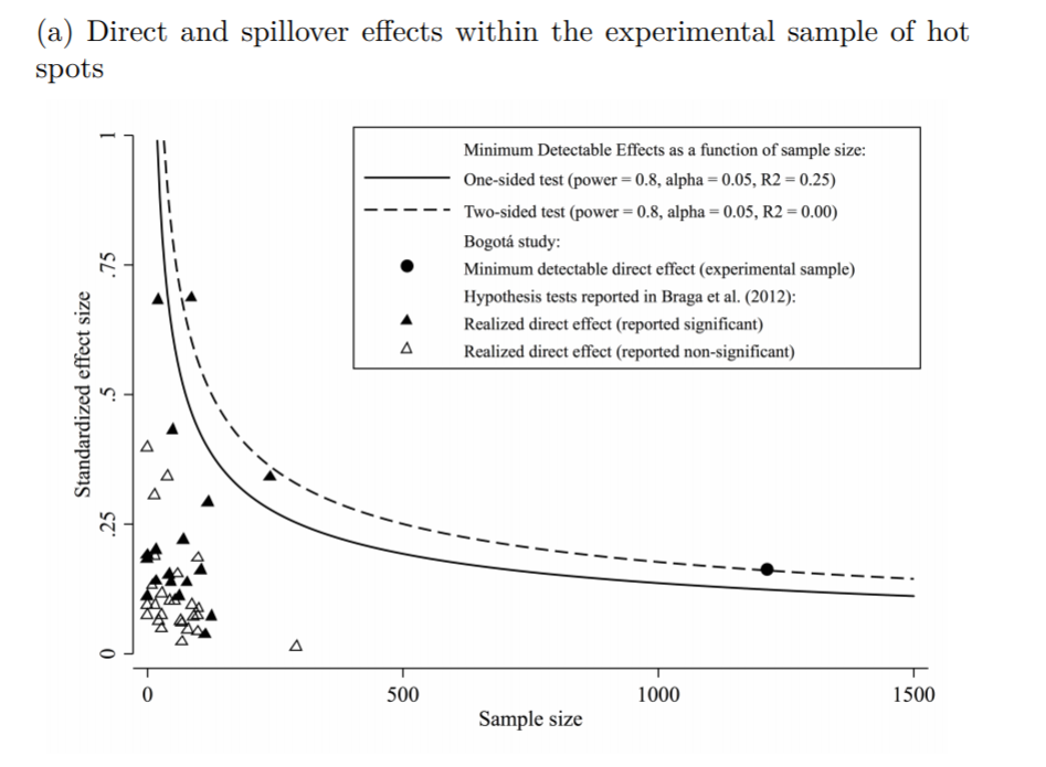
The line signifies a Cohen’s D of 0.17, and here is the same graph for the spillover estimates:

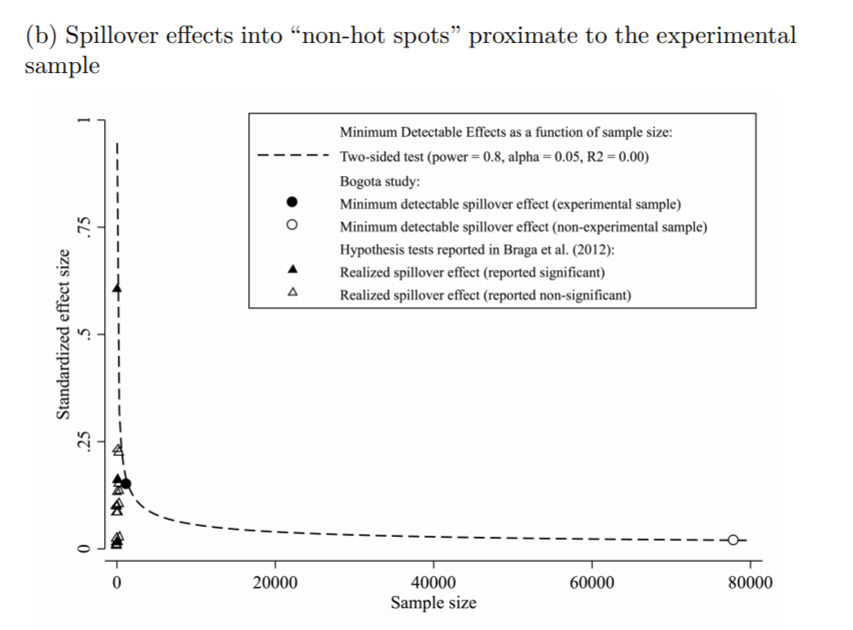
So you can see Blattman’s study in total number of spatial units of analysis breaks the chart so to speak. You can see however there are plenty of hot spot studies in either chart that reported statistically significant differences, but do not meet the 0.17 threshold in Chris’s chart. How can this be? Well, Chris is goal switching a bit here, he is saying using his estimator the studies appear underpowered. The original studies on the graph though did not necessarily use his particular estimator.

The best but not quite perfect analogy I can think of is this. Imagine I build a car that gets better gas mileage compared to the current car in production. Then someone critiques this as saying the materials that go into production of the car have worse carbon footprints, so my car is actually worse for the environment. It would be fine to argue a different estimate of total carbon footprint is reasonable (here Chris could argue his estimator is better than the ones the originally papers used). It is wrong though to say you don’t actually improve gas mileage. So it is wrong for Chris to say the original articles are underpowered using his estimator, they may be well powered using a different estimator.

Indeed, using either my WDD estimator (Wheeler & Ratcliffe, 2018) or Wilson’s log IRR estimator (Wilson, 2021), I will show how power does not grow with more experimental units, but with a larger baseline number of crimes for those estimators. They both only have two spatial units of analysis, so in Chris’s chart will never gain more power.

One way I think about the issue for spatial designs is this – you could always split up a spatial lattice into ever finer and finer spatial units of analysis. For example Chris could change his original design to use addresses instead of street segments, and split up the spillover buffers into finer slices as well. Do you gain something for doing nothing though? I doubt it.

I describe in my dissertation how finer spatial units of analysis allow you to check for finer levels of spatial spillovers, e.g. can check if crime spills over from the back porch to the front stoop (Wheeler, 2015). But when you do finer spatial units, you get more cold floor effects as well due to the limited nature of crime counts – they cannot go below 0. So designs with lower baseline crime rates tend to show lower power (Hinkle et al., 2013).

MDE for the WDD and log IRR

For minimum detectable effect (MDE) sizes for OLS type estimators, you need to specify the variance you expect the underlying treated/control groups to have. With the count type estimators I will show here, the variance is fixed according to the count. So all I need to specify is the alpha level of the test. Here I will do a default of 0.05 alpha level (with different lines for one-tailed vs two-tailed). The other assumption is the distribution of crime counts between treated/control areas. Here I assume they are all equal, so 4 units (pre/post and treated/control). For my WDD estimator this actually does not matter, for the later IRR estimator though it does (so the lines won’t really be exact for his scenario).

So here is the MDE for mine and Jerry’s WDD estimator:

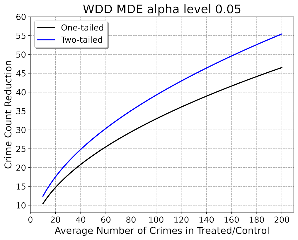
What this means is that if you have an average of 20 crimes in the treated/control areas for each time period separately, you would need to find a reduction of 15 crimes to meet this threshold MDE for a one-tailed. It is pretty hard when starting with low baselines! For an example close to this, if the treated area went from 24 to 9, and the control area was 24 to 24, this would meet the minimal treated reduction of 15 crimes in this example.

And here is the MDE for the log IRR estimator. The left hand Y axis has the logged effect, and the right hand side has the exponentiated IRR (incident rate ratio).

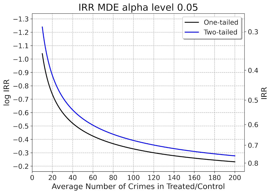
Since the IRR is commonly thought of as a percent reduction, this suggests even with baselines of 200 crimes, for Wilson’s IRR estimator you need percent reductions of over 20% relative to control areas.

So I have not gone through the more recent Braga et al. (2020) meta-analysis. I do not know if they have the data readily available to draw the points on this plot the same as in the Blattman article. To be clear, it may be Blattman is right and these studies are underpowered using either his or my estimator, I am not sure. (I think they probably are quite underpowered to detect spillover, since this presumably will be an even smaller amount than the direct effect. But that would not explain estimates of diffusion of benefits commonly found in these studies!)

I also do not know if one estimator is clearly better or not – for example Blattman could use my estimator if he simply pools all treated/control areas. This is not obviously better than his approach though, and foregoes any potential estimates of treatment effect variance (I will be damned if I can spell that word starting with het even close enough for autocorrect). But maybe the pooled estimate is OK, Blattman does note that he has cold floor effects in his linear estimator – places with higher baselines have larger effects. This suggests Wilson’s log IRR estimator with the pooled data may be just fine and dandy for example.

Python code

Here is the python code in its entirety to generate the above two graphs. You can see the two functions to calculate the MDE given an alpha level and average crime counts in each area if you are planning your own study, the wdd_mde and lirr_mde functions.

'''
Estimating minimum detectable effect sizes
for place based crime interventions

Andy Wheeler
'''

import numpy as np
from scipy.stats import norm
import matplotlib
import matplotlib.pyplot as plt
import os
my_dir = r'D:\Dropbox\Dropbox\Documents\BLOG\min_det_effect'
os.chdir(my_dir)

#########################################################
#Settings for matplotlib

andy_theme = {'axes.grid': True,
              'grid.linestyle': '--',
              'legend.framealpha': 1,
              'legend.facecolor': 'white',
              'legend.shadow': True,
              'legend.fontsize': 14,
              'legend.title_fontsize': 16,
              'xtick.labelsize': 14,
              'ytick.labelsize': 14,
              'axes.labelsize': 16,
              'axes.titlesize': 20,
              'figure.dpi': 100}

matplotlib.rcParams.update(andy_theme)
#########################################################

#########################################################
# Functions for MDE for WDD and logIRR estimator


def wdd_mde(avg_counts,alpha=0.05,tails='two'):
    se = np.sqrt( avg_counts*4 )
    if tails == 'two':
        a = 1 - alpha/2
    elif tails == 'one':
        a = 1 - alpha
    z = norm.ppf(a)
    est = z*se
    return est

def lirr_mde(avg_counts,alpha=0.05,tails='two'):
    se = np.sqrt( (1/avg_counts)*4 )
    if tails == 'two':
        a = 1 - alpha/2
    elif tails == 'one':
        a = 1 - alpha
    z = norm.ppf(a)
    est = z*se
    return est

# Generating regular grid from 10 to 200
cnts = np.arange(10,201)
wmde1 = wdd_mde(cnts, tails='one')
wmde2 = wdd_mde(cnts)

imde1 = lirr_mde(cnts, tails='one')
imde2 = lirr_mde(cnts)

# Plot for WDD MDE
fig, ax = plt.subplots(figsize=(8,6))
ax.plot(cnts, wmde1,color='k',linewidth=2, label='One-tailed')
ax.plot(cnts, wmde2,color='blue',linewidth=2, label='Two-tailed')
ax.set_axisbelow(True)
ax.set_xlabel('Average Number of Crimes in Treated/Control')
ax.set_ylabel('Crime Count Reduction')
ax.legend(loc='upper left')
plt.xticks(np.arange(0,201,20))
plt.yticks(np.arange(10,61,5))
plt.title("WDD MDE alpha level 0.05")
plt.savefig('WDD_MDE.png', dpi=500, bbox_inches='tight')

# Plot for IRR MDE
fig, ax = plt.subplots(figsize=(8,6))
ax2 = ax.secondary_yaxis("right", functions=(np.exp, np.log))
ax.plot(cnts,-1*imde1,color='k',linewidth=2, label='One-tailed')
ax.plot(cnts,-1*imde2,color='blue',linewidth=2, label='Two-tailed')
ax.set_axisbelow(True)
ax.set_xlabel('Average Number of Crimes in Treated/Control')
ax.set_ylabel('log IRR')
ax.set_ylim(-0.16, -1.34)
ax.legend(loc='upper right')
ax.set_yticks(-1*np.arange(0.2,1.31,0.1))
ax2.set_ylabel('IRR')
ax2.grid(False)
plt.xticks(np.arange(0,201,20))
plt.title("IRR MDE alpha level 0.05")
plt.savefig('IRR_MDE.png', dpi=500, bbox_inches='tight')

#########################################################

References

• Blattman, C., Green, D., Ortega, D., & Tobón, S. (2018). Place-based interventions at scale: The direct and spillover effects of policing and city services on crime (No. w23941). National Bureau of Economic Research.
• Braga, A. A., & Weisburd, D. L. (2020). Does Hot Spots Policing Have Meaningful Impacts on Crime? Findings from An Alternative Approach to Estimating Effect Sizes from Place-Based Program Evaluations. Journal of Quantitative Criminology, Online First.
• Hinkle, J. C., Weisburd, D., Famega, C., & Ready, J. (2013). The problem is not just sample size: The consequences of low base rates in policing experiments in smaller cities. Evaluation Review, 37(3-4), 213-238.
• Wheeler, A.P. (2015). What we can learn from small units of analysis. Dissertation, SUNY Albany.
• Wheeler, A.P., & Ratcliffe, J.H. (2018). A simple weighted displacement difference test to evaluate place based crime interventions. Crime Science, 7(1), 11.
• Wilson, D. B. (2021). The relative incident rate ratio effect size for count-based impact evaluations: When an odds ratio is not an odds ratio. Journal of Quantitative Criminology, Online First.