Updates on CRIME De-Coder and ASEBP

So I have various updates on my CRIME De-Coder consulting site, as well as new posts on the American Society of Evidence Based Policing Criminal Justician series.

CRIME De-Coder

Blog post, Don’t use percent change for crime data, use this stat instead. I have written a bunch here about using Poisson Z-scores, so if you are reading this it is probably old news. Do us all a favor and in your Compstat reports drop ridiculous percent change metrics with low baselines, and use 2 * ( sqrt(Current) - sqrt(Past) ).

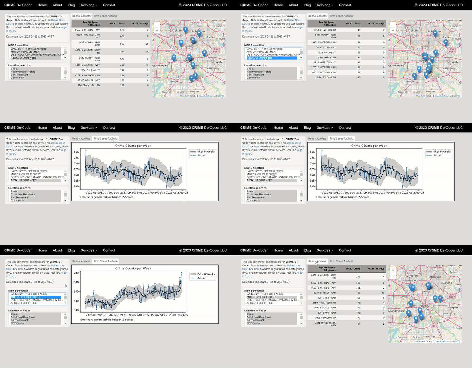
Blog post, Dashboards should be up to date. I will have a more techy blog post here on my love/hate relationship with dashboards (most of the time static reports are a better solution). But one scenario they do make sense is for public facing dashboards, but they should be up to date. The “free” versions of popular tools (Tableau, PowerBI) don’t allow you to link to a source dataset and get auto-updated, so you see many old dashboards out of date online. If you contract with me, I can automate it so it is up to date and doesn’t rely on an analyst manually updating the information.

Demo page – that page currently includes demonstrations for:

The WDD Tool is pure javascript – picking up more of that slowly (the Folium map has a few javascript listener hacks to get it to look the way I want). As a reference for web development, I like Jon Duckett’s three books (HTML, javascript, PHP).

Ultimately too much stuff to learn, but on the agenda are figuring out google cloud compute + cloud databases a bit more thoroughly. Then maybe add some PHP to my CRIME De-Coder site (a nicer contact me form, auto-update sitemap, and rss feed). I also want to learn how to make ArcGIS dashboards as well.

Criminal Justician

The newest post is Situational crime prevention and offender planning – discussing one of my favorite examples of crime prevention through environmental design (on suicide prevention) and how it is a signal about offender behavior that goes beyond simplistic impulsive behavior. I then relate this back to current discussion of preventing mass shootings.

If you have ideas about potential posts for the society (or this blog or crime de-coders blog), always feel free to make a pitch

Random notes, digital art, and pairwise comparisons is polynomial

So not too much in the hopper for the blog at the moment. Have just a bunch of half-baked ideas (random python tips, maybe some crime analysis using osmnx, scraping javascript apps using selenium, normal nerd data science stuff).

Still continuing my blog series on the American Society of Evidence Based Policing, and will have a new post out next week on officer use of force.

If you have any suggestions for topics always feel free to ask me anything!


Working on some random digital art (somewhat focused on maps but not entirely). For other random suggestions I like OptArt and Rick Wicklin’s posts.

Dall-E is impressive, and since it has an explicit goal of creating artwork I think it is a neat idea. Chat bots I have nothing good to say. Computer scientists working on them seem to be under the impression that if you build a large/good enough language model out pops general intelligence. Wee bit skeptical of that.


At work a co-worker was working on timing applications for a particular graph-database/edge-detection project. Initial timings on fake data were not looking so good. Here we have number of nodes and timings for the application:

  Nodes    Minutes
   1000       0.16
  10000       0.25
 100000       1.5
1000000      51

Offhand people often speak about exponential functions (or growth), but here what I expect is we are really looking at is pairwise comparisons (not totally familiar with the tech the other data scientist is using, so I am guessing the algorithmic complexity). So this likely scales something like (where n is the number of nodes in the graph):

Time = Fixed + C1*(n) + C2*(n choose 2) + e

Fixed is just a small constant, C1 is setting up the initial node database, and C2 is the edge detection which I am guessing uses pairwise comparisons, (n choose 2). We can rewrite this to show that the binomial coefficient is really polynomial time (not exponential) in terms of just the number of nodes.

C2*[n choose 2] = C2*[{n*(n-1)}/2]
                  C2*[ (n^2 - n)/2 ]
                  C2/2*[n^2 - n]
                  C2/2*n^2 - C2/2*n

And so we can rewrite our original equation in terms of simply n:

Time = Fixed + (C1 - C2/2)*N + C2/2*N^2

Doing some simple R code, we can estimate our equation:

n <- 10^(3:6)
m <- c(0.16,0.25,1.5,51)
poly_mod <- lm(m ~ n + I(n^2))

Since this fits 3 parameters with only 4 observations, the fit is (not surprisingly) quite good. Which to be clear does not mean much, if really cared would do much more sampling (or read the docs more closely about the underlying tech involved):

> pred <- predict(poly_mod)
> cbind(n,m,pred)
      n     m       pred
1 1e+03  0.16  0.1608911
2 1e+04  0.25  0.2490109
3 1e+05  1.50  1.5000989
4 1e+06 51.00 50.9999991

And if you do instead poly_2 <- lm(m ~ n + choose(n,2)) you get a change in scale of the coefficients, but the same predictions.

We really need this to scale in our application at work to maybe over 100 million records, so what would we predict in terms of minutes based on these initial timings?

> nd = data.frame(n=10^(7:8))
> predict(poly_mod,nd)/60 # convert to hours
         1          2
  70.74835 6934.56850

So doing 10 million records will take a few days, and doing 100 million will be close to 300 days.

With only 4 observations not much to chew over (really it is too few to say it should be a different model). I am wondering though how to best handle errors for these types of extrapolations. Errors are probably not homoskedastic for such timing models (error will be larger for larger number of nodes). Maybe better to use quantile regression (and model the median?). I am not sure (and that advice I think will also apply to modeling exponential growth as well).

Identifying near repeat crime strings in R or Python

People in criminology should be familiar with repeats or near-repeats for crimes such as robbery, burglaries, or shootings. An additional neat application of this idea though is to pull out strings of incidents that are within particular distance and time thresholds. See this example analysis by Haberman and Ratcliffe, The Predictive Policing Challenges of Near Repeat Armed Street Robberies. This is particularly useful to an analyst interested in crime linkage — to see if those particular strings of incidents are likely to be committed by the same offender.

Here I will show how to pluck out those near-repeat strings in R or Python. The general idea is to transform the incidents into a network, where two incidents are connected only if they meet the distance and time requirements. Then you can identify the connected components of the graph, and those are your strings of near-repeat events.

To follow along, here is the data and the code used in the analysis. I will be showing this on an example set of thefts from motor vehicles (aka burglaries from motor vehicles) in Dallas in 2015. In the end I take two different approaches to this problem — in R the solution will only work for smaller datasets (say n~5000 or less), but the python code should scale to much larger datasets.

Near-repeat strings in R

The approach I take in R does the steps as follows:

  1. compute the distance matrix for the spatial coordinates
  2. convert this matrix to a set of 0’s and 1’s, 1’s correspond to if the distance is below the user specified distance threshold (call it S)
  3. compute the distance matrix for the times
  4. convert this matrix to a set of 0’1 and 1’s, 1’s correspond to if the distance is below the user specified time threshold (call it T)
  5. use element-wise multiplication on the S and T matrices, call the result A, then set the diagonal of A to zero
  6. A is now an adjacency matrix, which can be converted into a network
  7. extract the connected components of that network

So here is an example of reading in the thefts from motor vehicle data, and defining my function, NearStrings, to grab the strings of incidents. Note you need to have the igraph R library installed for this code to work.

library(igraph)

MyDir <- "C:\\Users\\axw161530\\Dropbox\\Documents\\BLOG\\SourceNearRepeats"
setwd(MyDir)

BMV <- read.csv(file="TheftFromMV.csv",header=TRUE)
summary(BMV)

#make a function
NearStrings <- function(data,id,x,y,time,DistThresh,TimeThresh){
    library(igraph) #need igraph to identify connected components
    MyData <- data
    SpatDist <- as.matrix(dist(MyData[,c(x,y)])) < DistThresh  #1's for if under distance
    TimeDist <-  as.matrix(dist(MyData[,time])) < TimeThresh #1's for if under time
    AdjMat <- SpatDist * TimeDist #checking for both under distance and under time
    diag(AdjMat) <- 0 #set the diagonal to zero
    row.names(AdjMat) <- MyData[,id] #these are used as labels in igraph
    colnames(AdjMat) <- MyData[,id] #ditto with row.names
    G <- graph_from_adjacency_matrix(AdjMat, mode="undirected") #mode should not matter
    CompInfo <- components(G) #assigning the connected components
    return(data.frame(CompId=CompInfo$membership,CompNum=CompInfo$csize[CompInfo$membership]))
}

So here is a quick example run on the first ten records. Note I have a field that is named DateInt in the csv, which is just the integer number of days since the first of the year. In R though if the dates are actual date objects you can submit them to the dist function though as well.

#Quick example with the first ten records
BMVSub <- BMV[1:10,]
ExpStrings <- NearStrings(data=BMVSub,id='incidentnu',x='xcoordinat',y='ycoordinat',time='DateInt',DistThresh=30000,TimeThresh=3)
ExpStrings

So here we can see this prints out:

> ExpStrings
            CompId CompNum
000036-2015      1       3
000113-2015      2       4
000192-2015      2       4
000251-2015      1       3
000360-2015      2       4
000367-2015      3       1
000373-2015      4       2
000378-2015      4       2
000463-2015      2       4
000488-2015      1       3

The CompId field is a unique Id for every string of events. The CompNum field states how many events are within the string. So we have one string of events that contains 4 records in this subset.

Now this R function comes with a big caveat, it will not work on large datasets. I’d say your pushing it with 10,000 incidents. The issue is holding the distance matrices in memory. But if you can hold the matrices in memory this will still run quite fast. For 5,000 incidents it takes around ~15 seconds on my machine.

#Second example alittle larger, with the first 5000 records
BMVSub2 <- BMV[1:5000,]
BigStrings <- NearStrings(data=BMVSub2,id='incidentnu',x='xcoordinat',y='ycoordinat',time='DateInt',DistThresh=1000,TimeThresh=3)

The elements in the returned matrix will line up with the original dataset, so you can simply add those fields in, and do subsequent analysis (such as exporting back into a mapping program and digging into the strings).

#Add them into the original dataset
BMVSub2$CompId <- BigStrings$CompId
BMVSub2$CompNum <- BigStrings$CompNum   

You can check out the number of chains of different sizes by using aggregate and table.

#Number of chains
table(aggregate(CompNum ~ CompId, data=BigStrings, FUN=max)$CompNum)

This prints out:

   1    2    3    4    5    6    7    9 
3814  405   77   27    3    1    1    1

So out of our first 1,000 incidents, using the distance threshold of 1,000 feet and the time threshold of 3 days, we have 3,814 isolates. Thefts from vehicles with no other incidents nearby. We have 405 chains of 2 incidents, 77 chains of 3 incidents, etc. You can pull out the 9 incident like this since there is only one chain that long:

#Look up the 9 incident
BMVSub2[BMVSub2$CompNum == 9,]  

Which prints out here:

> BMVSub2[BMVSub2$CompNum == 9,]
      incidentnu xcoordinat ycoordinat StartDate DateInt CompId CompNum
2094 043983-2015    2460500    7001459 2/25/2015      56   1842       9
2131 044632-2015    2460648    7000542 2/26/2015      57   1842       9
2156 045220-2015    2461162    7000079 2/27/2015      58   1842       9
2158 045382-2015    2460154    7000995 2/27/2015      58   1842       9
2210 046560-2015    2460985    7000089  3/1/2015      60   1842       9
2211 046566-2015    2460452    7001457  3/1/2015      60   1842       9
2260 047544-2015    2460154    7000995  3/2/2015      61   1842       9
2296 047904-2015    2460452    7001457  3/3/2015      62   1842       9
2337 048691-2015    2460794    7000298  3/4/2015      63   1842       9

Or you can look up a particular chain by its uniqueid. Here is an example of a 4-chain set.

> #Looking up a particular incident chains
> BMVSub2[BMVSub2$CompId == 4321,]
      incidentnu xcoordinat ycoordinat StartDate DateInt CompId CompNum
4987 108182-2015    2510037    6969603 5/14/2015     134   4321       4
4988 108183-2015    2510037    6969603 5/14/2015     134   4321       4
4989 108184-2015    2510037    6969603 5/14/2015     134   4321       4
4993 108249-2015    2510037    6969603 5/14/2015     134   4321       4

Again, only use this function on smaller crime datasets.

Near-repeat strings in Python

Here I show how to go about a similar process in Python, but the algorithm does not calculate the whole distance matrix at once, so can handle much larger datasets. An additional note is that I exploit the fact that this list is sorted by dates. This makes it so I do not have to calculate all pair-wise distances – I will basically only compare distances within a moving window under the time threshold – this makes it easily scale to much larger datasets.

So first I use the csv python library to read in the data and assign it to a list with a set of nested tuples. Also you will need the networkx library to extract the connected components later on.

import networkx as nx
import csv
import math

dir = r'C:\Users\axw161530\Dropbox\Documents\BLOG\SourceNearRepeats'

BMV_tup = []
with open(dir + r'\TheftFromMV.csv') as f:
    z = csv.reader(f)
    for row in z:
        BMV_tup.append(tuple(row))

The BMV_tup list has the column headers, so I extract that row and then figure out where all the elements I need, such as the XY coordinates, the unique Id’s, and the time column are located in the nested tuples.

colnames = BMV_tup.pop(0)
print colnames
print BMV_tup[0:10]

xInd = colnames.index('xcoordinat')
yInd = colnames.index('ycoordinat')
dInd = colnames.index('DateInt')
IdInd = colnames.index('incidentnu')

Now the magic — here is my function to extract those near-repeat strings. Again, the list needs to be sorted by dates for this to work.

def NearStrings(CrimeData,idCol,xCol,yCol,tCol,DistThresh,TimeThresh):
    G = nx.Graph()
    n = len(CrimeData)
    for i in range(n):
        for j in range(i+1,n):
            if (float(CrimeData[j][tCol]) - float(CrimeData[i][tCol])) > TimeThresh:
                break
            else:
                xD = math.pow(float(CrimeData[j][xCol]) - float(CrimeData[i][xCol]),2)
                yD = math.pow(float(CrimeData[j][yCol]) - float(CrimeData[i][yCol]),2)
                d = math.sqrt(xD + yD)
                if d < DistThresh:
                    G.add_edge(CrimeData[j][idCol],CrimeData[i][idCol])
    comp = nx.connected_components(G)
    finList = []
    compId = 0
    for i in comp:
        compId += 1
        for j in i:
            finList.append((j,compId))
    return finList

We can then do the same test on the first ten records that we did in R.

print NearStrings(CrimeData=BMV_tup[0:10],idCol=IdInd,xCol=xInd,yCol=yInd,tCol=dInd,DistThresh=30000,TimeThresh=3)

And this subsequently prints out:

[('000378-2015', 1), ('000373-2015', 1), ('000113-2015', 2), ('000463-2015', 2), ('000192-2015', 2), ('000360-2015', 2), 
('000251-2015', 3), ('000488-2015', 3), ('000036-2015', 3)]

The component Id’s wont be in the same order as in R, but you can see we have the same results. E.g. the string with three incidents contains the Id’s 000251, 000488, and 000036. Note that this approach does not return isolates — incidents which have no nearby space-time examples.

Running this on the full dataset of over 14,000 incidents takes around 20 seconds on my machine.

BigResults = NearStrings(CrimeData=BMV_tup,idCol=IdInd,xCol=xInd,yCol=yInd,tCol=dInd,DistThresh=1000,TimeThresh=3)

And that should scale pretty well for really big cities and really big datasets. I will let someone who knows R better than me figure out workarounds to scale to bigger datasets in that language.
Scraping Meth Labs with Python

For awhile in my GIS courses I have pointed to the DEA’s website that has a list of busted meth labs across the county, named the National Clandestine Laboratory Register. Finally a student has shown some interest in this, and so I spent alittle time writing a scraper in Python to grab the data. For those who would just like the data, here I have a csv file of the scraped labs that are geocoded to the city level. And here is the entire SPSS and Python script to go from the original PDF data to the finished product.

So first off, if you visit the DEA website, you will see that each state has its own PDF file (for example here is Texas) that lists all of the registered labs, with the county, city, street address, and date. To turn this into usable data, I am going to do three steps in Python:

  1. download the PDF file to my local machine using urllib python library
  2. convert that PDF to an xml file using the pdftohtml command line utility
  3. use Beautifulsoup to parse the xml file

I will illustrate each in turn and then provide the entire Python script at the end of the post.

So first, lets import the libraries we need, and also note I downloaded the pdftohtml utility and placed that location as a system path on my Windows machine. Then we need to set a folder where we will download the files to on our local machine. Finally I create the base url for our meth labs.

from bs4 import BeautifulSoup
import urllib, os

myfolder = r'C:\Users\axw161530\Dropbox\Documents\BLOG\Scrape_Methlabs\PDFs' #local folder to download stuff
base_url = r'https://www.dea.gov/clan-lab' #online site with PDFs for meth lab seizures

Now to just download the Texas pdf file to our local machine we would simply do:

a = 'tx'
url = base_url + r'/' + a + '.pdf'
file_loc = os.path.join(myfolder,a)
urllib.urlretrieve(url,file_loc + '.pdf')

If you are following along and replaced the path in myfolder with a folder on your personal machine, you should now see the Texas PDF downloaded in that folder. Now I am going to use the command line to turn this PDF into an xml document using the os.system() function.

#Turn to xml with pdftohtml, does not need xml on end
cmd = 'pdftohtml -xml ' + file_loc + ".pdf " + file_loc
os.system(cmd)

You should now see that there is an xml document to go along with the Texas file. You can check out its format using a text editor (wordpress does not seem to like me showing it here).

So basically we can use the top and the left attributes within the xml to identify what row and what column the items are in. But first, we need to read in this xml and turn it into a BeautifulSoup object.

MyFeed = open(file_loc + '.xml')
textFeed = MyFeed.read()
FeedParse = BeautifulSoup(textFeed,'xml')
MyFeed.close()

Now the FeedParse item is a BeautifulSoup object that you can query. In a nutshell, we have a top level page tag, and then within that you have a bunch of text tags. Here is the function I wrote to extract that data and dump it into tuples.

#Function to parse the xml and return the line by line data I want
def ParseXML(soup_xml,state):
    data_parse = []
    page_count = 1
    pgs = soup_xml.find_all('page')
    for i in pgs:
        txt = i.find_all('text')
        order = 1
        for j in txt:
            value = j.get_text() #text
            top = j['top']
            left = j['left']
            dat_tup = (state,page_count,order,top,left,value)
            data_parse.append(dat_tup)
            order += 1
        page_count += 1
    return data_parse

So with our Texas data, we could call ParseXML(soup_xml=FeedParse,state=a) and it will return all of the data nested in those text tags. We can just put these all together and loop over all of the states to get all of the data. Since the PDFs are not that large it works quite fast, under 3 minutes on my last run.

from bs4 import BeautifulSoup
import urllib, os

myfolder = r'C:\Users\axw161530\Dropbox\Documents\BLOG\Scrape_Methlabs\PDFs' #local folder to download stuff
base_url = r'https://www.dea.gov/clan-lab' #online site with PDFs for meth lab seizures
                                           #see https://www.dea.gov/clan-lab/clan-lab.shtml
state_ab = ['al','ak','az','ar','ca','co','ct','de','fl','ga','guam','hi','id','il','in','ia','ks',
            'ky','la','me','md','ma','mi','mn','ms','mo','mt','ne','nv','nh','nj','nm','ny','nc','nd',
            'oh','ok','or','pa','ri','sc','sd','tn','tx','ut','vt','va','wa','wv','wi','wy','wdc']
            
state_name = ['Alabama','Alaska','Arizona','Arkansas','California','Colorado','Connecticut','Delaware','Florida','Georgia','Guam','Hawaii','Idaho','Illinois','Indiana','Iowa','Kansas',
              'Kentucky','Louisiana','Maine','Maryland','Massachusetts','Michigan','Minnesota','Mississippi','Missouri','Montana','Nebraska','Nevada','New Hampshire','New Jersey',
              'New Mexico','New York','North Carolina','North Dakota','Ohio','Oklahoma','Oregon','Pennsylvania','Rhode Island','South Carolina','South Dakota','Tennessee','Texas',
              'Utah','Vermont','Virginia','Washington','West Virginia','Wisconsin','Wyoming','Washington DC']

all_data = [] #this is the list that the tuple data will be stashed in

#Function to parse the xml and return the line by line data I want
def ParseXML(soup_xml,state):
    data_parse = []
    page_count = 1
    pgs = soup_xml.find_all('page')
    for i in pgs:
        txt = i.find_all('text')
        order = 1
        for j in txt:
            value = j.get_text() #text
            top = j['top']
            left = j['left']
            dat_tup = (state,page_count,order,top,left,value)
            data_parse.append(dat_tup)
            order += 1
        page_count += 1
    return data_parse

#This loops over the pdfs, downloads them, turns them to xml via pdftohtml command line tool
#Then extracts the data

for a,b in zip(state_ab,state_name):
    #Download pdf
    url = base_url + r'/' + a + '.pdf'
    file_loc = os.path.join(myfolder,a)
    urllib.urlretrieve(url,file_loc + '.pdf')
    #Turn to xml with pdftohtml, does not need xml on end
    cmd = 'pdftohtml -xml ' + file_loc + ".pdf " + file_loc
    os.system(cmd)
    #parse with BeautifulSoup
    MyFeed = open(file_loc + '.xml')
    textFeed = MyFeed.read()
    FeedParse = BeautifulSoup(textFeed,'xml')
    MyFeed.close()
    #Extract the data elements
    state_data = ParseXML(soup_xml=FeedParse,state=b)
    all_data = all_data + state_data

Now to go from those sets of tuples to actually formatted data takes a bit of more work, and I used SPSS for that. See here for the full set of scripts used to download, parse and clean up the data. Basically it is alittle more complicated than just going from long to wide using the top marker for the data as some rows are off slightly. Also there is complications for long addresses being split across two lines. And finally there are just some data errors and fields being merged together. So that SPSS code solves a bunch of that. Also that includes scripts to geocode the to the city level using the Google geocoding API.

Let me know if you do any analysis of this data! I quickly made a time series map of these events via CartoDB. You can definately see some interesting patterns of DEA concentration over time, although I can’t say if that is due to them focusing on particular areas or if they are really the areas with the most prevalent Meth lab problems.

https://andyw.carto.com/viz/882243de-ff69-11e6-b574-0e98b61680bf/public_map

Spatial join points to polygons using Python and SPSS

A recent use case of mine I had around 60 million points that I wanted to assign to census block groups. ArcGIS was being problematic to simply load in the 60 million point dataset (let alone spatial join it), so I wrote some python code and will show using python and SPSS how to accomplish this.

First, a shout out to Rex Douglass and this blog post, I’ve adapted most of the python code here from that example. Also before we get started, it will be necessary to download several geospatial libraries for python. Here you need shapely, pyshp, and rtree. As a note, I have only been able to get these to install and work using the IOOS channel for Anaconda, e.g. conda install -c ioos shapely rtree pyshp. (I have not been able to get fiona to work.)

The Python Part

So I will go through a quick rundown of the python code first. All of the data and code to run this yourself can be downloaded here. To start, I import all of the necessary libraries and functions.

import shapefile
from rtree import index
from shapely.geometry import Polygon, Point

The next step is to read in the polygon shapefile that we want to assign points to. Note you could swap this part out with fiona (if you can get it working!), but I just use the pyshp function shapefile.Reader. Note you need to change the data string to point to where the shapefile containing your polygons is located on your local machine.

#load in the shapefile of block groups
data = r'C:\Users\axw161530\Dropbox\Documents\BLOG\Point_inPoly_PythonSPSS'
bg_NYC = shapefile.Reader(data + r'\NYC_BG14_Proj.shp')

In my data these are block groups for New York city, and they are projected into feet using a local projection. (As an FYI, you can open up the “prj” file for shapefiles in a plain text editor to see the projection.) Now, the shapefile object, bg_NYC here, has several iterables that you can access either the geometries or the records available. First we need to get those individual polygons and stuff into a list, and then convert into a Polygon object shapely can deal with.

bg_shapes = bg_NYC.shapes()  #get the iterable for the polygon boundary points
bg_points = [q.points for q in bg_shapes] #convert to list of geometry
polygons = [Polygon(q) for q in bg_points] #convert to a shapely Polygon

Next I am going to do two things. First to make a vector that matches those Polygons to a particular id, I need to read in the data attributes from the shapefile. This is accomplished via the .records() attribute. For US census geometries they have what is oft labeled a GEOID. In this example shapefile the GEOID ends up being in the second variable slot. The second thing I accomplish here is I build an rtree lookup. The motivation for this is, when we do a point in polygon check, it can be an expensive procedure the more polygons you have. You can first limit the number of potential polygons to check though by only checking whether a point falls within the bounding box of a polygon, and then do the more expensive operation on the actual (more complicated) boundary of the polygon.

#build spatial index from bounding boxes
#also has a second vector associating area IDs to numeric id
bg_records = bg_NYC.records() #bg_records[0][1] is the geoid
idx = index.Index() #creating an rtree
c_id = 0
area_match = []
for a,b in zip(bg_shapes,bg_records):
    area_match.append(b[1])
    idx.insert(c_id,a.bbox,obj=b[1])
    c_id += 1

Now we have all the necessary ingredients to make a function that inputs one X,Y point, and then returns a GEOID. First, the function turns the input X,Y points into a Point object shapely can work with. Second, it does the bounding box lookup I mentioned earlier, using the idx rtree that is available in the global environment. Third, it loops over those resulting polygons that intersected the bounding box, and checks to see if the point is within that polygon using the shapely operation point.within(polygon). If that is true, it returns the associated GEOID, and if none are found it returns None. Again, the objects in this function idx, polygons, and area_match are taken from the global environment. A few additional notes: it will return the first point in polygon found, so if you have overlapping polygons this will simply return the first, not necessarily all of them. That is not the case with our census polygons here though. Second, the functionality here is for a point on the exact border between two polygons to return False.

#now can define function with polygons, area_match, and idx as globals
def assign_area(x,y):
    point = Point(x,y)
    for i in idx.intersection((x,y,x,y)): 
        if point.within(polygons[i]):
            return area_match[i]
    return None
#note points on the borders will return None

To test this function I have a set of points in New York for this particular projection already associated with a GEOID.

#now testing
test_vec = [(1003610, 239685, '360050063002'),
            (1006787, 240666, '360050183022'),
            ( 993580, 219484, '360610122001'),
            ( 986385, 214971, '360610115001'),
            ( 947148, 167688, '360850201001'),
            (      0,      0, 'Miss')]

for a,b,c in test_vec:
    print [assign_area(x=a,y=b),c]

And this should subsequently print out at your console:

['360050063002', '360050063002']
['360050183022', '360050183022']
['360610122001', '360610122001']
['360610115001', '360610115001']
['360850201001', '360850201001']
[None, 'Miss']

For those wishing to do this in vectorized in python, check out the GeoPanda’s functionality. But here I let it churn out one by one by using SPSS.

The SPSS Part

So once the above function is defined in your SPSS environment, we can simply use SPSSINC TRANS to assign XY data to a block group. Here is a quick example. First we read in some data, this is the homicide data from the New York times discussed here. It has the points projected in the same feet as the polygons were.

*Conducting point in polygon tests with Python and SPSS.
FILE HANDLE data /NAME = "C:\Users\axw161530\Dropbox\Documents\BLOG\Point_inPoly_PythonSPSS".
*Read in the NYC homicide data.
GET TRANSLATE FILE='data\HomPoints_JoinBG.dbf' /TYPE=DBF /MAP .
DATASET NAME HomData.

Now I am going to use the SPSS command SHOW to display the current date and time, (so you can see how long the operation takes). This dataset has 4,021 cases of homicide, and the set of polygons we are matching to has around 6,500 block groups. The time the operation takes depends on both, but the rtree search should make the number of polygons not as big a deal as simply looping through all of them. Second, I use SPSSINC TRANS to call the python function we previously constructed. Third, this dataset already has the GEOID matched to the points (via ArcGIS), so I check to make sure I get the same results as ArcGIS. In this example there are quite a few points that ArcGIS failed to return a match for, but this operation does. (It would take more investigation on my part though as to why that is the case.)

*Use this to show timing.
SHOW $VAR.

*Now using SPSSINC TRANS to assign geoid.
SPSSINC TRANS RESULT=GeoID2 TYPE=12
  /FORMULA "assign_area(x=XFt,y=YFt)".

SHOW $VARS.
*Check that the operations are all correct (as compared to ArcGIS)
COMPUTE Check = (GEOID = GEOID2).
FREQ Check.

This example runs almost instantly. For some tests with my bigger dataset of 60 million, matching half a million points to this set of polygons took around 12 minutes.

To End

Again, all of the data and code to run this at once can be downloaded here. I will need to make a blog post at some point of using pyproj to project point data in SPSS as well, such as to go to and from Lat-Lon to a local projection. You probably always want to do geometric operations like this and buffers with projected data, but you may get the data in Lat-Lon or want to export data in Lat-Lon to use online maps.

For those working with crime data, I oft complain that crime is frequently on the borders of census geographies. But due to slight differences in resolution, most GIS systems will still assign crime points to census geographies. I’m not sure if it is a big problem for much analysis in our field, but the proportion on the border is clearly quite large in some instances. For things that can occur often outdoors, like robberies and field stops, the proportion is even higher because crime is often recorded at intersections (I have estimates for the percentage of crimes at intersections for 14 years in Albany in this paper). So the problem depends on the crime type or nature of the incident (traffic stops are almost always listed at intersections), but I have seen analysis I would bet over 50% of the incidents are on the border of census blocks and/or block groups.

A general way to check this in GIS is to turn your polygon data into lines, and then assign points to the nearest line and check the distance. You will see many points that are very close to the border (say within 5 meters) that really should be undetermined.

Downloading and reading in American Community Survey Data: Python and SPSS

I had a prior blog post on working with American Community Survey data in SPSS. The meta-data format has changed from that example though, and the Census gives out comma separated files and xls Templates now. So this will be an update, and I have good stuff for those working strictly in python, as well as those wanting to load the data is SPSS.

So first, when downloading the small geographies from the Census’s FTP site, they have a ton of files. See this page, which contains the 5 year estimates for 2014 for New York block groups and tracts. Now instead of downloading each zip file one by one, we can write a quick python script to download all the files.

import urllib, os

downFold = r'C:\Users\axw161530\Dropbox\Documents\BLOG\ACS_Python_SPSS\Data'
base = r'http://www2.census.gov/programs-surveys/acs/summary_file/2014/data/5_year_seq_by_state/NewYork/Tracts_Block_Groups_Only/'

for i in range(1,5):  #change range(1,5) to range(1,122) to download all zip files
    file = "20145ny0" + str(i).zfill(3) + "000.zip"
    urllib.urlretrieve(base + file, os.path.join(downFold,file))

#also download the geography file
urllib.urlretrieve(base + "g20145ny.csv", os.path.join(downFold,"g20145ny.csv"))

The downFold string is where the files will be downloaded to (so change that to a place on your local machine), and the base string ends up being the base URL for that particular set of files. The files go from 1 to 121 in that example, but just to keep the time down I only download tables one through four. The second urlib.urlretrieve line downloads the geography csv file (we won’t be using the other geography file, which is the same data but in tab delimited format).

Now we can go and download the meta data excel file shells. For this dataset they are located here. Here we want the 5 year templates. Once that data is downloaded, then unzip all of the files. You could technically do this in python as well, but I just use 7zip, as that has a handy dialog to unzip multiple files to the same place.

So the way the files work, there are a set of estimate and margin of error text files that are comma delimited that have the demographic characteristics. (Here for all block groups and census tracts in New York.) The xls excel files contain the variable names, along with a brief description for the variables.

If you are a hipster and only do data analysis in python, here is a function that takes the location to a xls template file and the corresponding data file and reads it into a pandas data frame.

#this reads in american community survey data
import xlrd
import pandas as pd

def readACS(Template,Data):
    book = xlrd.open_workbook(Template) #first open the xls workbook
    sh = book.sheet_by_index(0)
    vars = [i.value for i in sh.row(0)] #names on the first row
    labs = [i.value for i in sh.row(1)] #labels on the second
    #this rewrites duplicate 'BLANK' names, mangle dups not working for me
    n = 0
    vars2 = []
    for i in range(len(vars)):
        if vars[i] == 'BLANK':
            n += 1
            vars2.append('BLANK.' + str(n))
        else:
            vars2.append(vars[i])
    #check for if geo file or data file
    if vars2[1] == 'FILETYPE':
        df = pd.read_csv(Data,names=vars2,dtype={'FILETYPE':'object'})
    else:
        df = pd.read_csv(Data,names=vars2)
    return df,zip(vars2,labs)

In a nutshell, it reads the metadata column names and labels from the excel spreadsheet, then reads in the csv file with the data. It returns two objects, the one on the left is a pandas dataframe, and the one on the right is a zipped up list of the variable names and the variable labels. This would be a bit simpler, except that the format for the geo dataset is a little different than all the data files and contains multiple “BLANK” fields (the mangle_dupe_cols option in read_csv is not behaving like I expect it to). For the non-geographic file, I need to tell python the filetype column is a string, else it interprets the “e” in the estimate files as a scientific number (e.g. 1e5 = 100,000).

So here is an example of using this function to grab the second table. When I unzipped the excel templates, it nested the data templates in another subfolder, hence the TemplateFold string.

TemplateFold = downFold + r'\seq'
Tab002,Meta002 = readACS(TemplateFold + r'\Seq2.xls',downFold + r'\e20145ny0002000.txt')

If you want to check out all the variable labels, you can then do:

for i in Meta002:
    print i 

Or if you want to turn that into a dictionary you can simply do dict(Meta002). If you wanted to import all 121 tables and merge them you should be able to figure that out in a simple loop from here (note the “x.zfill(n)” function to pad the integers with leading zeroes). But I typically only work with a select few tables and variables at a time, so I won’t worry about that here.

The function works the same with the geographic data and its template. (Which that metadata template is not nested in the further down seq folder.)

GeoDat,MetaGeo = readACS(downFold + r'\2014_SFGeoFileTemplate.xls',downFold + r'\g20145ny.csv')

Note if you are working with both the estimates and the margin of error files, you may want to put somewhere in the code to change the variable names to signify that, such as by putting a suffix of “e” or “m”. If you just work with the estimates though you don’t need to worry about that.

Reading ACS data into SPSS

For those working in SPSS, I’ve shown previously how to turn python data into SPSS data. I’ve started working on a function to make this simpler with pandas dataframes, but I will hold off on that for now (need to figure out datetimes and NaN’s). So what I did here was grab the meta-data from the template xls file (same as before), but from that build the necessary DATA LIST command in SPSS, and then just submit the command. SPSS has the added benefit of having native meta-data fields, so I can also add in the variable labels. Also, this only uses the xlrd library, in case you do not have access to pandas. (I point SPSS to Anaconda, instead of worrying about using pip with the native SPSS python install.)

So in SPSS, you would first define this function

*This just builds the necessary SPSS program to read in the american community survey data.
BEGIN PROGRAM Python.
#creating my own function to read in data
import xlrd, spss
def OpenACS(Template,Data):
  book = xlrd.open_workbook(Template)
  sh = book.sheet_by_index(0)
  vars = [i.value for i in sh.row(0)]
  labs = [i.value for i in sh.row(1)]
  #this rewrites duplicate 'BLANK' names, mangle dups not working for me
  n = 0
  vars2 = []
  for i in range(len(vars)):
    if vars[i] == 'BLANK':
      n += 1
      vars2.append('BLANK.' + str(n))
    else:
      vars2.append(vars[i])
    #check for if geo file or data file
  if vars2[1] == 'FILETYPE':  #regular data
    ncols = sh.ncols - 6 #need the end of the number of variables
    ext =  ' (' + str(ncols) + 'F7.0)'
    v1 = ' /FILEID FILETYPE (2A6) STUSAB (A2) CHARITER (A3) SEQUENCE (A4) LOGRECNO (A7) '
    v2 = '\n '.join(vars2[6:])
    Tab = Data[-10:-7] #Names the dataset based on the table number
  else: #geo data file
    ncols = sh.ncols
    ext =  ' (' + str(ncols) + 'A255)' #255 should be big enough to fit whatever str
    v1 = " / "
    v2 = '\n '.join(vars2)
    Tab = "Geo"
  #this sets errors off, implicit missing data for block groups
  spss.Submit("PRESERVE.")
  spss.Submit("SET RESULTS OFF ERRORS OFF.")
  #now creating the import program to read in the data
  begin = "DATA LIST LIST(',') FILE = '%s'" % (Data)
  full_str = begin + v1 + v2 + ext + "\n."
  #now reading in the dataset
  spss.Submit(full_str)
  #assigning a dataset name
  datName = "DATASET NAME Table" + Tab + "." 
  spss.Submit(datName)
  #now adding in the variable labels
  for i,j in zip(vars2,labs):
    #replaces double quotes with single quotes in label
    strVal = """VARIABLE LABELS %s "%s".""" % (i,j.replace('"',"'"))
    spss.Submit(strVal)
  if Tab == "Geo":
    spss.Submit("ALTER TYPE ALL (A = AMIN).")
  spss.Submit("RESTORE.")
END PROGRAM.

Again this is much shorter if I only needed to worry about the data files and not the geo file, but that slight formatting difference is a bit of a pain. Here I use the errors off trick to suppress the data list errors for missing data (which is intended, as not all of the data is available at the block group level). But you will still get error messages in the SPSS syntax bottom section. They can be ignored if it is the “insufficient data” warning.

Here is an example of using this python function now to read the data into SPSS. This automatically assigns a dataset name, either based on the Table number, or “Geo” for the geographic data.

*Now reading in the data files I want.
BEGIN PROGRAM Python.
downFold = r'C:\Users\axw161530\Dropbox\Documents\BLOG\ACS_Python_SPSS\Data'
TemplateFold = downFold + r'\seq'

#reading in Data file, table number 2
OpenACS(TemplateFold + r'\Seq2.xls',downFold + r'\e20145ny0002000.txt')

#reading in Geo file
OpenACS(downFold + r'\2014_SFGeoFileTemplate.xls',downFold + r'\g20145ny.csv')
END PROGRAM.
EXECUTE.

And Voila, there is your small area American Community Survey data in SPSS. This will produce two different datasets, “Table002” and “TableGeo” that can be merged together via MATCH FILES.

Let me know in the comments if you have already worked out a function to turn pandas dataframes into SPSS datasets.

Added code snippets page

I’ve written quite a few blog posts over the years, and it is getting to be hard for me to keep all of them orderly. So I recently created a page with a simple table of contents with code snippets broken down into categories. There are also a few extra SPSS macros in there that I have not written blog posts about.

Every now and then I see a broken link and update it, but I know there are more I am missing. So just send an email if I have a link to some of my code and it is currently broken.


Sentence length in academic articles

While reviewing a paper recently it struck me that the content was (very) good, but the writing was stereotypical academic. My first impression was that this was caused by monotonously long sentences. See this advice from Gary Provost (via Francis Diebold). Part of the reason why long sentences are undesirable is not only for aesthetic reasons though — longer sentences are harder to parse, hold in memory, and subsequently understand. See Steven Pinker’s The Sense of Style writing guide for discussion.

So I did some text analysis of the sentences. To do the text analysis I used the nltk library in python, and here is the IPython notebook to replicate for yourself if you care to do so (apparently Wakari is not a thing anymore, so here is the corpus for Huck Finn and for my Small Sample paper). In the notebook I have saved two text corpuses, one my finished draft of this article. I compared the sentence length to Mark Twain’s Huckleberry Finn (text via here).

For a simple example getting started with the library, here is an example of tokenizing a string into words and sentences:

#some tests for http://www.nltk.org/, nice book to follow along
import nltk
#nltk.download('punkt') #need to download this for the English sentence tokenizer files

#this splits up punctuation
test = """At eight o'clock on Thursday morning Arthur didn't feel very good. This is a second sentence."""
tokens = nltk.word_tokenize(test)
print tokens

ts = nltk.sent_tokenize(test)
print ts

The first prints out each individual word (plus punctuation in some circumstances) and the second marks individual sentences. I have the line #nltk.download('punkt') commented out, as I downloaded it once already. (Running once in Wakari I did not need to download it again – I presume it would work similarly on your local machine.)

So what I did was transfer the PDF document I was reviewing to a text file and then clean up things like the section headers (ditto for my academic articles I compare it to). In Huckleberry I took out the table of contents and the “CHAPTER ?” parts. I also started a list of variables that were parsed as words but that I did not want to count after the sentences and words were tokenized. For example, an inline cite such as (X, 1996) would be split into 4 words with the original tokenizer, (, X, 1996 and ). The “x96” is an en-dash. Below takes those instances out.

#Get the corpus
f = open('SmallSample_Corpus.txt')
raw = f.read()

#Count number of sentences
sent_tok = nltk.sent_tokenize(raw)
ns = len(sent_tok)

#Count number of words
word_tok = nltk.word_tokenize(raw) #need to take out commas plus other stuff
NoWord = [',','(',')',':',';','.','%','\x96','{','}','[',']','!','?',"''","``"]
word_tok2 = [i for i in word_tok if i not in NoWord]
nw = len(word_tok2)

#Average Sentence length are words divided by sentences
print float(nw)/ns

There are inevitably more instances of things that shouldn’t be counted as words, but that makes the sentences longer on average. For example, I spotted a few possessive 's that were listed as different words. (The nltk library is smart and lists contractions as seperate words.)

So someone may know a better way to count the words, but all the articles should have the same biases. In my tests, here are the average number of words per sentence:

  • article I was reviewing, 28
  • my small sample article, 27
  • my working article (that has not undergone review), 25
  • Huck Finn, 20

So the pot is calling the kettle black here – my writing is not much better. I looked at the difference between an in-print article and a working draft, as responses to reviewers I bet will make the sentences longer. Hedges in statements that academics love.

Looking at the academic article histograms they are fairly symmetric, confirming my impression about monotonous sentence length. To make the histograms I used the panda’s library, which has a nice simple method.

sent_len = []
for i in sent_tok:
    sent_w1 = nltk.word_tokenize(i)
    sent_w2 = [i for i in sent_w1 if i not in NoWord]
    sent_len.append(len(sent_w2))

import pandas as pd

dfh = pd.DataFrame(sent_len)
dfh.hist(bins = 50);

Here is the histogram for my small sample paper:

And here it is for Huck Finn

(I’m not much of an exemplar for making graphs in python – forgive the laziness in the figures.) Apparently analyzing sentence length has a long history, see a paper by G. Udny Yule in 1939! From a quick perusal the long right tail is more usual for analyzing texts. The symmetry I see for this sample of academic articles is not the norm.

There could be more innocuous reasons for this. Huck Finn has dialogue with shorter sentences, and the academic articles have numbers and citations. (Although I think it is reasonable to count those things towards sentence complexity, “1” or “one” should have the same complexity.)

I will have to keep this in mind in the future (maybe I should write my articles in poem form)!

Neighborhoods in Albany according to Google

One of the most vexing aspects of spatial analysis in the social sciences in the concept of neighborhoods. There is a large literature on neighborhood effects in criminology, but no one can really define a neighborhood. For analysis they are most often assumed to approximately conform to census areas (like tracts or blocks). Sometimes there are obvious physical features that divide neighborhoods (most often a major roadway), but more often boundaries are fuzzy.

I’ve worked on several surveys (at the Finn Institute) in which we ask people what neighborhood they live in as well as the nearest intersection to their home. Even where there is a clear border, often people say the “wrong” neighborhood, especially near the borders. IIRC, when I calculated the wrongness for one survey in Syracuse we did it was only around 60% of the time the respondents stated they lived the right neighborhood. I do scare quotes around “wrong” because it is obviously arbitrary where people draw the boundaries, so more people saying the wrong neighborhood is indicative of the borders being misaligned than the respondents being wrong.

For this reason I like the Google maps approach in which they just place a label at the approximate center of noteworthy neighborhoods. I emulated this for a recent background map I made for a paper in Albany. (Maps can be opened in a separate tab to see a larger image.)

As background I did not grow up in Albany, but I’ve lived and worked in the Capital District since I came up to Albany for grad school – since 2008. Considering this and the fact that I make maps of Albany on a regular basis is my defense I have a reasonable background to make such judgements.

When looking at Google’s reverse geocoding API the other day I noticed they returned a neighborhood field in the response. So I created a regular sampling grid over Albany to see what they return. First, lets see my grid and where Google actually decides some neighborhood exists. Large grey circles are null, and small red circles some neighborhood label was returned. I have no idea where Google culls such neighborhood labels from.

See my python code at the end of the post to see how I extracted this info. given an input lat-lng. In the reverse geo api they return multiple addresses – but I only examine the first returned address and look for a neighborhood. (So I could have missed some neighborhoods this way – it would take more investigation.)

Given the input fishnet I then dissolved the neighborhood labels into areas. Google has quite a few more specific neighborhoods than me.

I’ve never really made much of a distinction between West Hill and Arbor Hill – although the split is clearly at Henry Johnson. Also I tend to view Pine Hill as the triangle between Western and Central before the State campus – but Google and others seem to disagree with me. What I call the Pinebush Google calls the Dunes. Dunes is appropriate, because it actually has sand dunes, but I can’t recall anyone referring to it as that. Trees are pretty hard to come by in Arbor Hill though, so don’t be misled. Also kill is Dutch for creek, so you don’t have to worry that Normanskill is such a bad place (even if your name is Norman).

For a third opinion, see albany.com

You can see more clearly in this map how Pine Hill’s area goes south of Madison. Google maps has a fun feature showing related maps, and so they show a related map on someones take for where law students should or should not get an apartment. In that map you can see that south of Madison is affectionately referred to as the student ghetto. That comports with my opinion as well, although I did not think putting student ghetto was appropriate for my basemap for a journal article!

People can’t seem to help but shade Arbor Hill in red. Which sometimes may be innocent – if red is the first color used in defaults (as Arbor Hill will be the first neighborhood in an alphabetic list). But presumably the law student making the apartment suggestions map should know better.

In short, it would be convenient for me (as a researcher) if everyone could agree with what a neighborhood is and where its borders are, but that is not reality.


Here is the function in Python to grab the neighborhood via the google reverse geocoding API. Here if it returns anything it grabs the first address returned and searches for the neighborhood in the json. If it does not find a neighborhood it returns None.

#Reverse geocoding and looking up neighborhoods
import urllib, json

def GoogRevGeo(lat,lng,api=""):
  base = r"https://maps.googleapis.com/maps/api/geocode/json?"
  GeoUrl = base + "latlng=" + str(lat) + "," + str(lng) + "&key=" + api
  response = urllib.urlopen(GeoUrl)
  jsonRaw = response.read()
  jsonData = json.loads(jsonRaw)
  neigh = None
  if jsonData['status'] == 'OK':
    for i in jsonData['results'][0]['address_components']:
      if i['types'][0] == 'neighborhood':
        neigh = i['long_name']
        break
  return neigh

Using the Google Geocoding API with Python

Previously I posted how to use the geopy python library to call the Google geocode API. But somewhere along the way my version of geopy was not working (maybe because the API changed). Instead of figuring out that problem, I just wrote my own function to call the Google API directly. No need to worry about installing geopy.

Part of the reason I blog is so I have notes for myself – I’m pretty sure I’ve rewritten this several times for different quick geocoding projects, but I couldn’t find them this morning when I needed to do it again. So here is a blog post for my own future reference.

Here is the function, it takes as input the full string address. Also I was getting back some null responses by rapid fire calling the API (with only 27 addresses), so I set the function to delay for five seconds and that seemed to fix that problem.

import urllib, json, time
def GoogGeoAPI(address,api="",delay=5):
  base = r"https://maps.googleapis.com/maps/api/geocode/json?"
  addP = "address=" + address.replace(" ","+")
  GeoUrl = base + addP + "&key=" + api
  response = urllib.urlopen(GeoUrl)
  jsonRaw = response.read()
  jsonData = json.loads(jsonRaw)
  if jsonData['status'] == 'OK':
    resu = jsonData['results'][0]
    finList = [resu['formatted_address'],resu['geometry']['location']['lat'],resu['geometry']['location']['lng']]
  else:
    finList = [None,None,None]
  time.sleep(delay) #in seconds
  return finList

And here is an example use of the function. It returns the formatted address, the latitude and the longitude.

#Example Use
test = r"1600 Amphitheatre Parkway, Mountain View, CA"
geoR = GoogGeoAPI(address=test)
print geoR

This works for a few addresses without an API key. Even with an API key though the limit I believe is 2,500 – so don’t use this to geocode a large list. Also if you have some special characters in your address field this will take more work. For example if you have an & for an intersection I bet this url call will fail. But that should not be too hard to deal with. Also note the terms of service for using the API (which I don’t understand – so don’t ask me!)

I should eventually wrap up all of this google API python code into an extension for SPSS. Don’t hold your breath though for me getting the time to do that.


Here is an update for Python 3+ (the urllib library changed a bit). Also shows how to extract out the postal code.

#Update For Python 3+
#Also includes example parsing out the postal code
import urllib.request, urllib.parse 
import json, time
key = r'???!!!your key here!!!!????'

def GoogGeoAPI(address,api="",delay=3):
  base = r"https://maps.googleapis.com/maps/api/geocode/json?"
  addP = "address=" + urllib.parse.quote_plus(address)
  GeoUrl = base + addP + "&key=" + api
  response = urllib.request.urlopen(GeoUrl)
  jsonRaw = response.read()
  jsonData = json.loads(jsonRaw)
  if jsonData['status'] == 'OK':
    resu = jsonData['results'][0]
    post_code = -1
    for i in resu['address_components']:
      if i['types'][0] == 'postal_code':
        post_code = i['long_name'] #not sure if everything always has a long name?
    finList = [resu['formatted_address'],resu['geometry']['location']['lat'],resu['geometry']['location']['lng'],post_code]
  else:
    finList = [None,None,None,None]
  time.sleep(delay) #in seconds
  return finList
  
test = r"1600 Amphitheatre Parkway, Mountain View, CA"
geoR = GoogGeoAPI(address=test,api=key,delay=0)
print(geoR)