Haven’t gotten the time to publish a blog post in a few. There has been a ton of stuff I have put out on my Crime De-Coder website recently. For some samples since I last mentioned here, have published four blog posts:
- on what AI regulation in policing would look like
- high level advice on creating dashboards
- overview of early warning systems for police
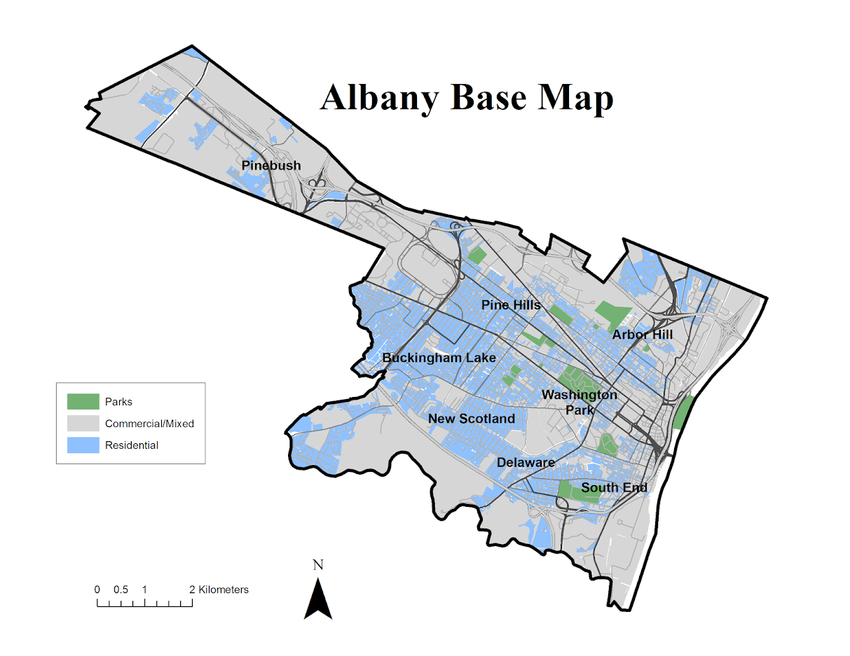
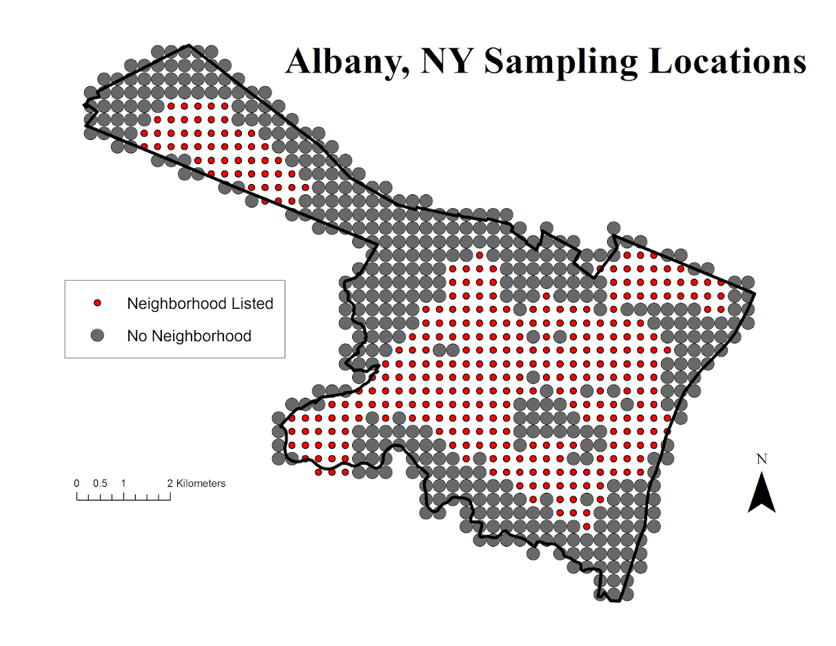
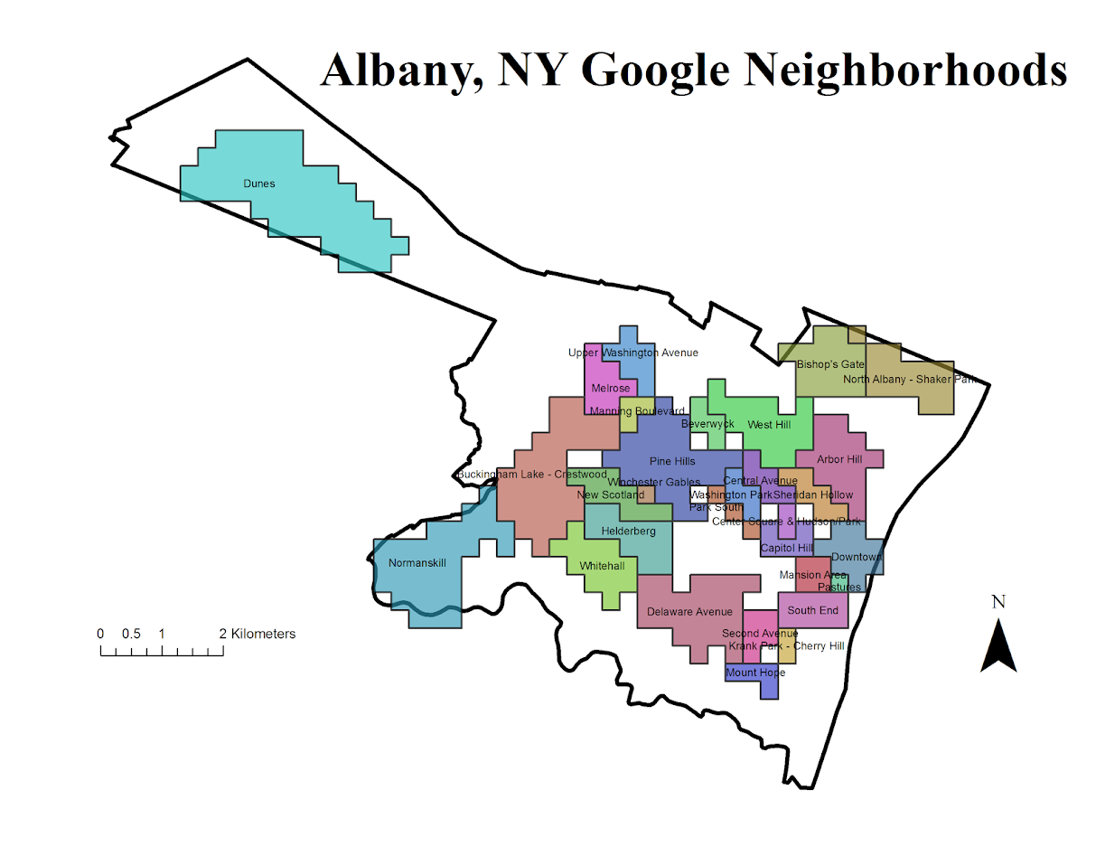
- types of surveys for police departments
For surveys a few different groups have reached out to me in regards to the NIJ measuring attitudes solicitation (which is essentially a follow up of the competition Gio and myself won). So get in touch if interested (whether a PD or a research group), may try to coordinate everyone to have one submission instead of several competing ones.
To keep up with everything, my suggestion is to sign up for the RSS feed on the site. If you want an email use the if this than that service. (I may have to stop doing my AltAc newsletter emails, it is so painful to send 200 emails and I really don’t care to sign up for another paid for service to do that.)
I also have continued the AltAc newsletter. Getting started with LLMs, using secrets, advice on HTML, all sorts of little pieces of advice every other week.
I have created a new page for presentations. Including, my recent presentation at the Carolina Crime Analysis Association Conference. (Pic courtesy of Joel Caplan who was repping his Simsi product – thank you Joel!)

If other regional IACA groups are interested in a speaker always feel free to reach out.
And finally a new demo on creating a static report using quarto/python. It is a word template I created (I like often generating word documents that are easier to post-hoc edit, it is ok to automate 90% and still need a few more tweaks.)
Harmweighted Hotspots
If you like this blog, also check out Iain Agar’s posts, GIS/SQL/crime analysis – the good stuff. Here I wanted to make a quick note about his post on weighting Crime Harm spots.
So the idea is that when mapping harm spots, you could have two different areas with same high harm, but say one location had 1 murder and one had 100 thefts. So if murder harm weight = 100 and theft harm weight = 1, they would be equal in weight. Iain talks about different transformations of harm, but another way to think about it is in terms of variance. So here assuming Poisson variance (although in practice that is not necessary, you could estimate the variance given enough historical time series data), you would have for your two hotspots:
Hotspot1: mean 1 homicide, variance 1
Hotspot2: mean 100 thefts, variance 100

Weight of 100 for homicides, 1 for theft

Hotspot1: Harmweight = 1*100 = 100
          Variance = 100^2*1 = 10,000
          SD = sqrt(10,000) = 100

Hotspot2: Harmweight = 100*1 = 100
          Variance = 1^2*100 = 100
          SD = sqrt(100) = 10
When you multiply by a constant, which is what you are doing when multiplying by harm weights, the relationship with variance is Var(const*x) = const^2*Var(x). The harm weights add variance, so you may simple add a penalty term, or rank by something like Harmweight - 2*SD (so the lower end of the harm CI). So in this example, the low end of the CI for Hotspot 1 is 0, but the low end of the CI for Hotspot2 is 80. So you would rank Hotspot2 higher, even though they are the same point estimate of harm.
The rank by low CI is a trick I learned from Evan Miller’s blog.
You could fancy this up more with estimating actual models, having multiple harm counts, etc. But this is a quick way to do it in a spreadsheet with just simple counts (assuming Poisson variance). Which I think is often quite reasonable in practice.
Using ESRI Python API
So I knew you could use python in ESRI, they have a notebook interface now. What I did not realize is now with Pro you can simply do pip install arcgis, and then just interact with your org. So for a quick example:
from arcgis.gis import GIS

# Your ESRI url
gis = GIS("https://modelpd.maps.arcgis.com/", username="user_email", password="???yourpassword???")
# For batch geocoding, probably need to do GIS(api_key=<your api key>)
This can be in whatever environment you want, so you don’t even need ArcGIS installed on the system to use this. It is all web-api’s with Pro. To geocode for example, you would then do:
from arcgis.geocoding import geocode, Geocoder, get_geocoders, batch_geocode

# Can search to see if any nice soul has published a geocoding server

arcgis_online = GIS()
items = arcgis_online.content.search('geocoder north carolina', 'geocoding service', max_items=30)

# And we have four
#[<Item title:"North Carolina Address Locator" type:Geocoding Layer owner:ecw31_dukeuniv>,
# <Item title:"Southeast North Carolina Geocoding Service" type:Geocoding Layer owner:RaleighGIS>,
# <Item title:"Geocoding Service - AddressNC " type:Geocoding Layer owner:nconemap>,
# <Item title:"ArcGIS World Geocoding Service - NC Extent" type:Geocoding Layer owner:NCDOT.GOV>]

geoNC = Geocoder.fromitem(items[0]) # lets try Duke
#geoNC = Geocoder.fromitem(items[-1]) # NCDOT.GOV
# can also do directly from URL
# via items[0].url
# url = 'https://utility.arcgis.com/usrsvcs/servers/8caecdf6384144cbafc9d56944af1ccf/rest/services/World/GeocodeServer'
# geoNC = Geocoder(url,gis)

# DPAC
res = geocode('123 Vivian Street, Durham, NC 27701',geocoder=geoNC, max_locations=1)
print(res[0])
Note you cannot cache the geocoding results. To do that, you need to use credits and probably sign in via a token and not a username password.
# To cache, need a token
r2 = geocode('123 Vivian Street, Durham, NC 27701',geocoder=geoNC, max_locations=1,for_storage=True)

# If you have multiple addresses, use batch_geocode, again need a token
#dc_res = batch_geocode(FullAddressList, geocoder=geoNC)
Geocoding to this day is still such a pain. I will need to figure out if you can make a local geocoding engine with ESRI and then call that through Pro (I mean I know you can, but not sure pricing for all that).
Overall being able to work directly in python makes my life so much easier, will need to dig more into making some standard dashboards and ETL processes using ESRI’s tools.
I have another post that has been half finished about using the ESRI web APIs, hopefully will have time to put that together before another 6 months passes me by!