Faking synthetic control estimates

AI disclosure – this post was created via Claude Code using Claude Opus 5 on xhigh reasoning effort. I gave it the idea, the data, the estimator and my prior blog posts as style examples, and it wrote the code and the draft. I will always disclose when I use AI to heavily write any content on this blog. (I use it for minor copy editing all the time.)

A few years back I wrote some notes on the Hogan/Kaplan back and forth. Short version, Tom Hogan used synthetic control to say Larry Krasner’s de-prosecution caused extra homicides in Philadelphia (Hogan, 2022), and Jacob Kaplan, JJ Naddeo and Tom Scott said the result was an artifact of a very short pre-period and a few other specification choices (Kaplan et al., 2026). I thought KNS had the better of the substantive argument. But the thing that has stuck in my head for three years is not the substance, it is that Hogan never released his data or his code. Which meant every attempt at replication ended with no, the data you have are wrong.

Progressive prosecutors are the place in criminology where this bites hardest. It is a live political fight, the effect sizes people claim are enormous, and nearly every candidate jurisdiction has three or four other things going on at the same time. Los Angeles is the poster child. George Gascon was sworn in as LA County DA on December 7th, 2020, but California also had AB 109 realignment in 2011, Prop 47 in 2014 (raising the felony theft threshold to $950), and Prop 57 in 2016. Pick your intervention.

So here is the point of this post. It is not simply that you cannot check someone’s work when they withhold data and code. It is that a researcher who withholds data and code can report whatever post-intervention trajectory they want, and every diagnostic that appears in the paper will look completely normal. The pre-period fit, the table of donor weights, the significance test, the graph. All of it.

I am going to show this with four synthetic control models for monthly thefts in Los Angeles. Three of them are fabricated – one showing no effect, one showing a large increase, one showing a large decrease – and one is honest. Data and code are on github.

To be clear about what I am and am not saying, I have no reason to think Hogan or anybody else in this literature made up numbers. My claim is about what the published record can and cannot rule out. If the only thing standing between a result and fabrication is the author’s say-so, that is not a standard of evidence, it is a character reference.

The setup

For the estimator I use the lasso plus conformal inference approach I have written about before, originally here and then applied to opioid deaths in Oregon and Washington here. You fit a lasso with non-negative coefficients to the treated unit’s pre-period series, using the comparison cities as predictors, and then get prediction intervals out of leave-one-out conformity scores. I like it better than the original Abadie optimizer, and the intervals tend to be tighter than placebo-based tests for state and city level designs.

The data are monthly thefts from the Real-Time Crime Index, which I already had a local snapshot of for another project. I keep agencies with a complete monthly series from January 2017 through November 2024, and use thefts per 100,000. That is 47 pre-period months and 48 post-period months, which is Gascon’s entire term.

For the donor pool I drop San Francisco, Chicago, Philadelphia and New York, since those all have DAs who wore the same label over the same window. I also have to drop the LA County Sheriff’s Department, because Gascon prosecuted its cases too – it is treated, not a control. That leaves 577 comparison agencies.

import FakeSynth
import LassoSynth
import pandas as pd

theft = pd.read_csv('LATheft.csv',parse_dates=['Date'])
wide = LassoSynth.prep_longdata(theft,'Date','Rate','City')

# Jan 2017 - Nov 2020 is the pre-period, so period 47 is Dec 2020
real = LassoSynth.Synth(wide,'Los Angeles, CA',47,alpha=30)
real.fit()
real.weights_table()

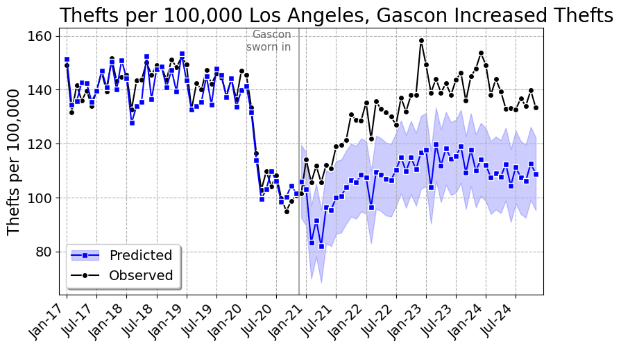
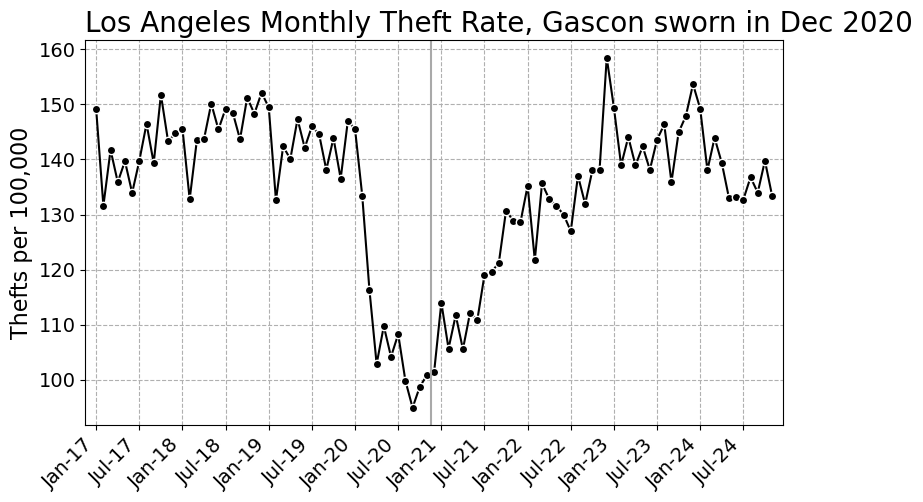
Here is the series we are trying to explain. The pandemic dent is obvious, and Gascon’s swearing in lands almost exactly at the bottom of it, which is its own problem.
The fake

The honest estimator fits the donor weights to the pre-period only. Everything after the vertical line is out of sample. Faking it means fitting the weights to all the periods, where you have replaced the treated unit’s post-period values with whatever you would like to publish. The pre-period values you leave alone, so the pre-period diagnostics stay honest looking.

The substantive change is three lines. Here are the guts of FakeSynth.py:

class FakeSynth(LassoSynth.Synth):
    def __init__(self,data,y,post,fake,alpha=1.0):
        super().__init__(data,y,post,alpha)
        # X is the same, the donor cities are real data
        self.fitX = pd.concat([self.preX,self.postX],axis=0)
        # y is real pre-period, whatever you want post-period
        fs = pd.Series(np.asarray(fake),index=self.postY.index,name=y)
        self.fitY = pd.concat([self.preY,fs],axis=0)
    def fit(self):
        # only difference, fit on all the periods
        self.mapie.estimator.fit(self.fitX,self.fitY)
        self.mapie.fit(self.fitX,self.fitY)
        # pre-period diagnostics versus the real pre-period data
        y_pred = self.mapie.predict(self.preX,ensemble=False)
        ...

And writing down the three stories takes one line each. For no effect, the synthetic Los Angeles should land on top of the observed data. For an increase, it should sit below. For a decrease, above.

obs_post = wide['Los Angeles, CA'].iloc[47:].to_numpy()

fakes = {'Fake null': obs_post*1.00,
         'Fake increase': obs_post*0.80,   # synthetic 20% under observed
         'Fake decrease': obs_post*1.25}   # synthetic 25% over observed

No effect

fake = FakeSynth.FakeSynth(wide,'Los Angeles, CA',47,obs_post*1.00,alpha=30)
fake.fit()
# {'RMSE': 4.85, 'RSquare': 0.913}
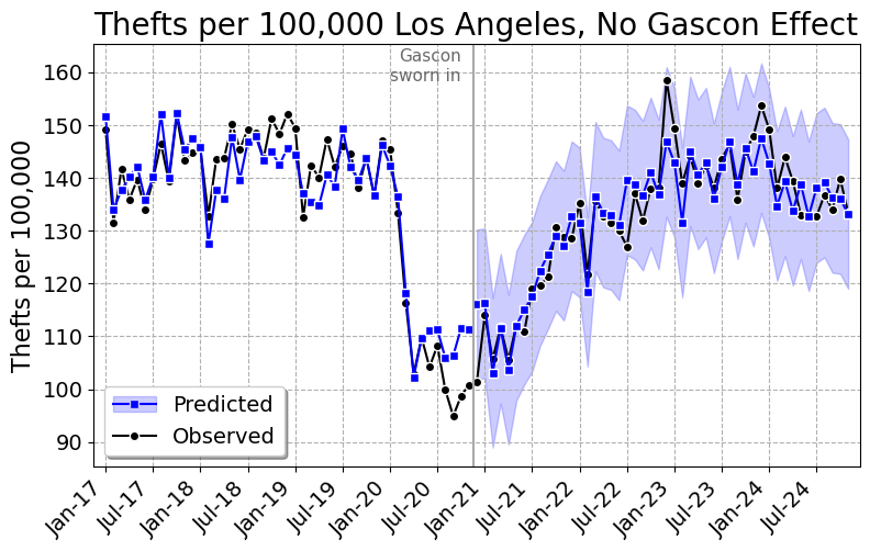
Pre-period R-square of 0.91, and the synthetic tracks LA right through the post period. Cumulative effect of 3 thefts per 100,000 over four years, 95% interval of -88 to 87. Gascon did nothing. Here are the ten largest weights, out of 27 that are non-zero:

City Weight
Intercept 37.1923
Alpharetta, GA 0.0780
Hayward, CA 0.0672
Miami, FL 0.0629
Baltimore, MD 0.0531
Vacaville, CA 0.0439
Paterson, NJ 0.0439
Wayne Township, NJ 0.0397
Baldwin Park, CA 0.0350
Detroit, MI 0.0328
Porterville, CA 0.0237

Gascon increased thefts

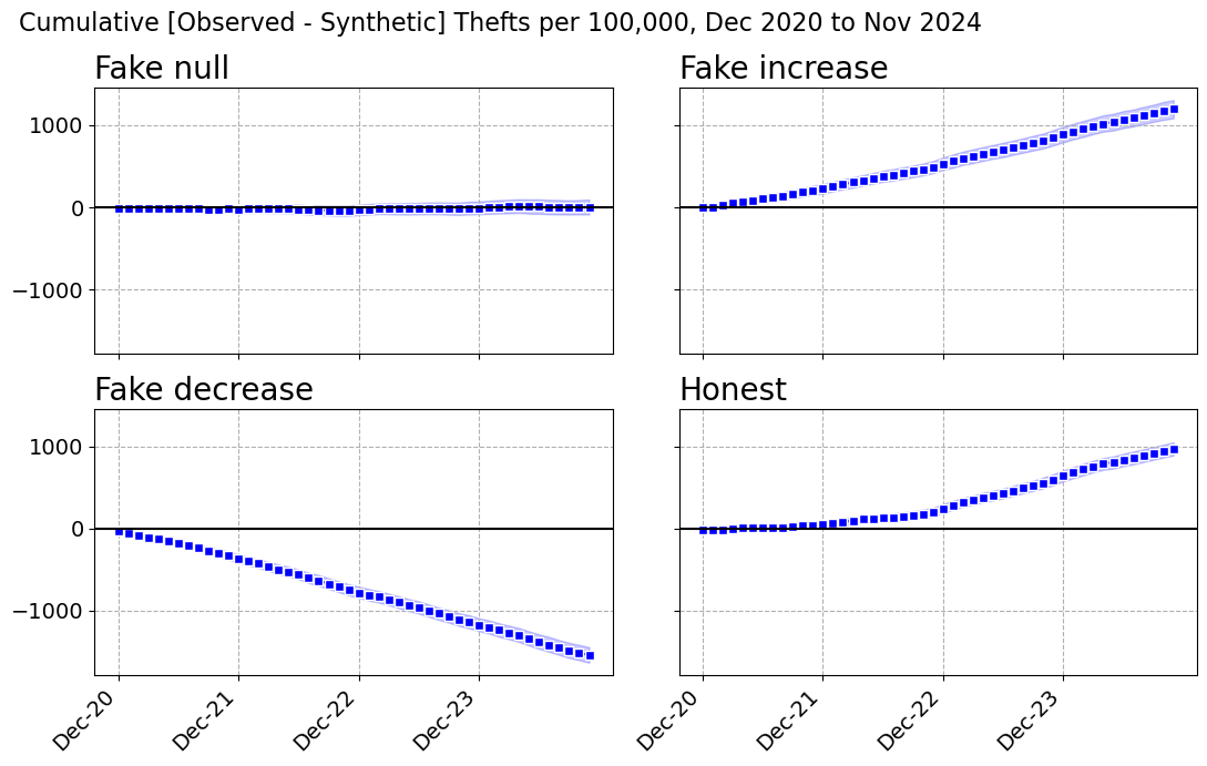
Pre-period R-square of 0.92, and the gap opens up right at December 2020 and never closes. That is +23.2%, a cumulative 1,199 thefts per 100,000, which given LA’s population is about 46,000 extra thefts over Gascon’s term. The 95% interval is 1,091 to 1,313. If you wanted a number for a press release, there it is.

City Weight
Intercept 6.6812
Laredo, TX 0.1313
Vacaville, CA 0.0542
Hayward, CA 0.0541
Novato, CA 0.0449
Antioch, CA 0.0432
Baltimore, MD 0.0369
Aiken Cnty, SC 0.0364
McAllen, TX 0.0362
Harlingen, TX 0.0360
Baldwin Park, CA 0.0337

Gascon decreased thefts

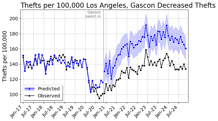
Same data, same code, same pre-period. -19.5%, or 59,662 thefts prevented, with a 95% interval that comfortably excludes zero. Pre-period R-square of 0.87. Gascon the crime fighter.

City Weight
Intercept 19.0633
Vallejo, CA 0.1618
Gardena, CA 0.0962
Arcadia, CA 0.0891
Paterson, NJ 0.0882
Alpharetta, GA 0.0625
Miami, FL 0.0467
Hayward, CA 0.0418
Baltimore, MD 0.0391
Frisco, TX 0.0380
Folsom, CA 0.0340

All four at once

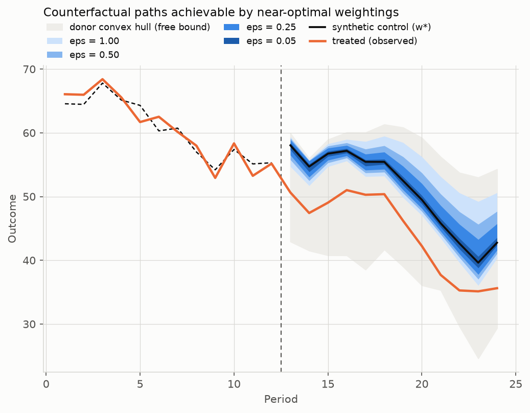
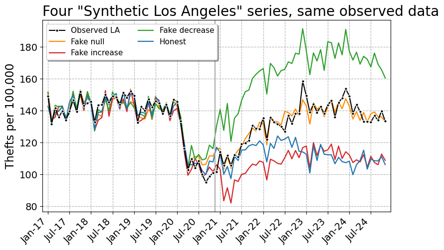
Here is what the fabrication looks like when you put the three fakes and the honest model on one set of axes. Identical observed data, identical donor pool, identical software. Four “synthetic Los Angeles” series that sit on top of each other in the pre-period and are 54 per 100,000 apart in the final month.
And the cumulative effect graphs, which is what actually ends up in the paper:
Model Pre RMSE Pre R2 Donors Monthly per 100k Percent Cumulative per 100k 95% CI Total Thefts
Fake null 4.85 0.913 27 0.1 0.0% 3 -88 to 87 108
Fake increase 4.55 0.924 31 25.0 23.2% 1,199 1,091 to 1,313 46,470
Fake decrease 5.88 0.872 22 -32.1 -19.5% -1,540 -1,640 to -1,442 -59,662
Honest 3.52 0.954 16 20.2 18.0% 972 900 to 1,041 37,644

There is exactly one number in that table that separates the fakes from the honest model, and it is the pre-period fit. The honest model does a little better, R-square 0.954 versus 0.872 to 0.924. That is because the fabricated model has to fit the real pre-period and the made up post-period simultaneously, so at a fixed penalty it gives up a bit of pre-period accuracy.

Which is not a tell you can use, for two reasons. First, nobody reading the paper knows what pre-period fit was achievable. Second, the fabricator can just turn the penalty down:

alpha Honest RMSE Honest R2 Faked RMSE Faked R2 Faked Percent
1 0.55 0.999 2.71 0.973 24.5%
5 1.57 0.991 3.27 0.961 24.2%
10 2.09 0.984 3.76 0.948 23.9%
20 2.92 0.969 4.22 0.934 23.5%
30 3.52 0.954 4.55 0.924 23.2%

At alpha=1 the fabricated model has a pre-period R-square of 0.973 – better than the honest model at the penalty I actually used – and still reports a 24.5% increase. You cannot referee your way out of this.

It is also worth killing the obvious partial remedy. “Fine, don’t release the microdata, just publish your weights.” That does not help at all. I took the published fake weights, multiplied them by the public donor data, and recovered the reported synthetic series to 13 decimal places. A replicator checking the weights against the donor data will confirm the figure exactly. The only thing that would catch this is re-estimating the weights from the pre-period, and that needs the donor pool, the data vintage, the tuning parameter and the software version – every one of which is something the original author can dispute after the fact. Which is precisely the Hogan situation.

The real answer

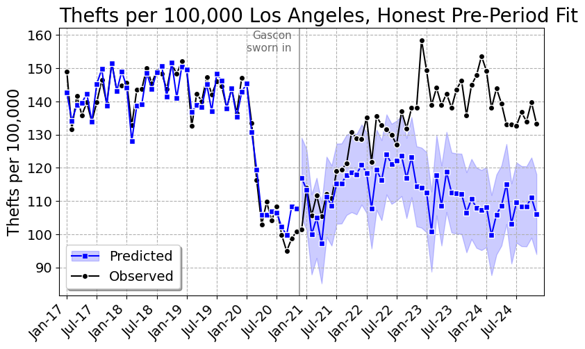
Now the honest model, weights fit on January 2017 through November 2020 only, everything after that out of sample.
City Weight
Intercept 22.2752
Laredo, TX 0.0965
Tucson, AZ 0.0928
Concord, CA 0.0782
Fairfield, CA 0.0726
Rock Hill, SC 0.0327
Baltimore, MD 0.0249
Portsmouth, VA 0.0238
Bakersfield, CA 0.0217
Santa Clara, CA 0.0179
Schaumburg, IL 0.0177

LA thefts run about 18% above the synthetic estimate, a cumulative 972 per 100,000 or roughly 37,600 extra thefts. So the honest answer in my preferred specification is in the same direction, and about three quarters the size, as the increase I made up.

I do not believe that number, and neither should you. Look at the graph, and at the gap by year:

Year Observed Synthetic Difference
2020 (Dec) 101.5 117.0 -15.5
2021 117.3 111.8 5.5
2022 134.8 118.5 16.3
2023 143.7 110.7 33.0
2024 137.6 107.7 29.9

That is a gap that starts negative, crosses zero sometime in 2021, and then grows for two straight years. It is not what a policy change that happened in December 2020 looks like. It is what a slow divergence in trend looks like, and a synthetic control cannot tell those apart. And here is what the estimate does when you poke it:

Spec Donors Percent Cumulative per 100k Total Thefts
Rates, all donors, alpha=5 38 15.0% 832 32,237
Rates, all donors, alpha=10 29 16.7% 912 35,321
Rates, all donors, alpha=20 22 18.1% 975 37,784
Rates, all donors, alpha=30 16 18.0% 972 37,644
Rates, all donors, alpha=50 12 15.8% 870 33,709
Rates, all donors, alpha=80 11 12.6% 710 27,524
Rates, 250k+ donors, alpha=10 13 9.7% 561 21,731
Rates, 250k+ donors, alpha=30 9 11.2% 643 24,911
Counts, all donors, alpha=30 43 5.3% n/a 12,381
Placebo Dec 2018 (12 mo), alpha=30 9 -3.9% -69 -2,690

The penalty barely matters, 13% to 18% across a sixteen-fold range of alpha. Two other things matter a lot. Restricting the donor pool to cities over 250,000 – on the grounds that Rock Hill, South Carolina is not a plausible counterfactual for Los Angeles – cuts it to about 10%. And doing it in counts instead of rates, which is the exact thing Hogan and KNS fought over, cuts it to 5.3%.

The last row is the one that should really bother you. Pretend Gascon took office in December 2018, throw away everything after November 2019, and refit. You get a statistically significant 4% decrease in thefts, over a year in which Jackie Lacey was DA and nothing in particular happened. If the design can find a four percent effect where there is nothing to find, an 18% estimate over a window containing a pandemic, an LAPD that shed more than a thousand officers, and a change in LAPD’s records system is not measuring a district attorney.

So my honest answer is: somewhere between 5% and 18%, with a failed placebo, and I would not put it in a paper. Which is the unsatisfying part. The fabricated numbers in this post are cleaner, tighter and more publishable than the real one. That is the incentive problem, and it is why “trust me, I’d rather not share the data” cannot be an acceptable answer.

Nerd Notes

The prediction intervals in the fabricated models come from conformity scores computed over all 95 periods, including the invented ones. So they are conditional on the fabrication and a bit narrower than they should be. If you cared about not leaving that particular fingerprint, you would compute the conformity scores from the pre-period only, which is another two lines.

I used a flat proportional shift because it is the simplest thing to explain. A more careful fabricator would use a phase-in – say a ramp over the first twelve months and then flat – because instantaneous discontinuities at the treatment date look suspicious to a reader who has seen a lot of these graphs. The lasso fits that just as happily. You can make the counterfactual any shape you like, including one where the effect conveniently only shows up in year three.

Nothing here is specific to synthetic control. Any method where the counterfactual is a fitted object – interrupted time series, matching, DiD with unit specific trends, an ML forecast – can be run backwards from the answer you want. Synthetic control is just an unusually comfortable place to do it, because it is a pure curve-fitting exercise with a large number of free parameters and a professional convention of reporting pre-period fit as the main validity check. Here I have 577 donors and 47 pre-period months. Drop the penalty to essentially zero and the pre-period R-square is 0.9999998, which should tell you how much that fit statistic is really worth.

There is a spillover issue I left in on purpose. Gascon prosecuted cases for every police department in LA County, so Long Beach, Pasadena, Pomona, Torrance and about thirty others in the donor pool are treated units. If Gascon actually moved thefts, leaving them in biases the estimate toward zero. I dropped the Sheriff’s Department – it polices about 945,000 residents of the county and shares the name in the data – but left the rest, and the code has a note about it. Same for Boston, Baltimore, St. Louis and Austin, all of which have a decent claim to the progressive prosecutor label over this window. Note that Baltimore City shows up in all four weights tables above.

The RTCI data are monthly counts as reported, and reporting practices are not stable. LAPD cut over to a new records management system starting March 7th, 2024, phased across bureaus through May, to comply with the FBI’s NIBRS-only mandate. LAPD’s own announcement warned the new format “may give the impression of increased crime levels.” That is inside my post period. To its credit, it does not look like it is driving anything here – the gap was already 33 per 100,000 through 2023 and it shrinks slightly in 2024 – but it is the kind of thing that a synthetic control on other cities cannot fix and that I would not have known about if I had not gone looking.

The repo has the full weights tables and the month by month effects for all four models as CSVs, not just the top ten I printed here. PrepGasconData.py builds the analysis file from the RTCI snapshot, FakeSynth.py is the fabrication, and GasconAnalysis.py makes every table and figure in this post. You will need mapie on top of the usual scientific python stack.

Finally, a defense that would actually work: preregister the donor pool and the estimator, then post the data and code. Both. If you will not post the code, you have not published a result, you have published an assertion with graphs.

References

Join CrimConsortium, ASEBP submissions open, VerusCite privacy, NACA Course

I have minor updates for several activities.

First, the American Society of Evidence-Based Policing is accepting submissions for its conference in spring 2027 at UPenn:

If you are a vendor interested in promoting some of your work at the conference, also feel free to get in touch. I serve on the committee that works with vendors and the committee that reviews proposals.

Second, I have updated several of the pages for Crim Consortium (roughly the nonprofit behind CrimRXiv).

For individuals, you should consider becoming a member to support the work Scott (and to a lesser extent myself) is doing on this. (We do not make money to be clear, just keeping the lights on.)

If you are a program head for a department (or involved in some other organization), you should consider becoming an institutional member. You get your own prioritized page (which is worth it just for the SEO for your group).

CrimRXiv has over a million pageviews per month at the moment. It is easily the best preprint server to post your work to for anything related to criminology at all. It is also the only preprint server that lets you upload your work in HTML format (you can upload a Markdown or LaTeX file as well and it turns the paper into HTML). So you can have embedded interactive graphics if you want, for example.

Third, VerusCite has a blog with the most recent post about How VerusCite Handles Privacy. For individuals running journals, I only submit the references to the LLMs, unlike other editors. Those LLMs are zero-data-retention, and I also do not see what you upload.

Journals should really be investing in my tool. Most journals would only take a few hundred per year at $2 per paper.

This is a major problem across science as a whole at the moment. The Hall of Hallucinations is up to 27 papers as of this writing, and I tend to add at least one a day.

Fourth, I have contributed a course to the new National Association of Crime Analysts called Basics of Python Programming for Crime Analysts.

This asynchronous course consists of bite-sized labs to go with my book, Data Science for Crime Analysis with Python. If you would like in-person training, get in touch, but this is much more economical for those interested in pursuing training on their own.

Crime De-Coder and VerusCite Updates

If you do not follow me on social media (X, LinkedIn), you likely have missed the different work I have been up to. So this is a remix of some of that, posted here for folks to follow along.

Crime De-Coder Blog

On the Crime De-Coder Blog:

I often debate whether to post things here or on the Crime De-Coder blog. So if you like my posts here, you should probably also follow Crime De-Coder. As you can see, it is a mix of recent technical and crime-analysis-related posts.

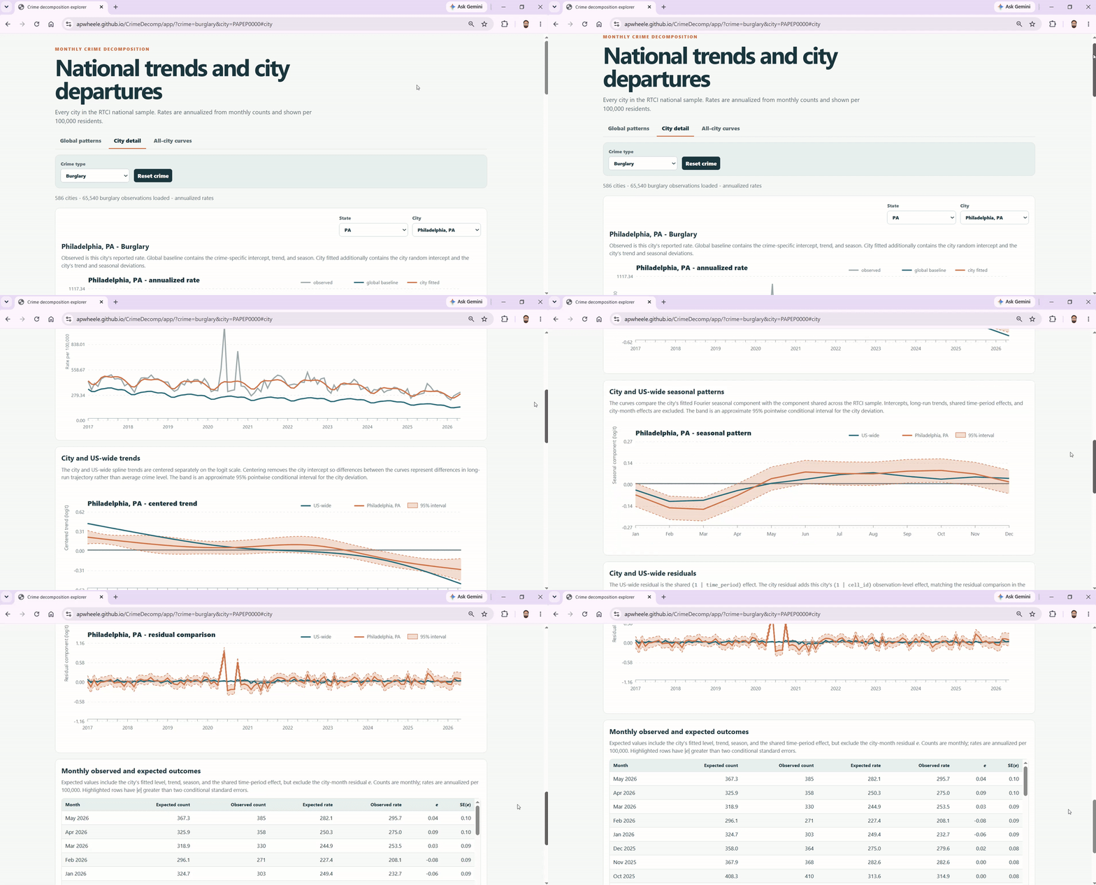
For the crime trends work, also check out my web app, where you can filter and compare cities relative to national trends (based on the Real-Time Crime Index data).

Note that I will be going to the Council on CJ working group on crime trends, on the causes of the homicide decline, in a few weeks, so let me know if you want to meet up.

VerusCite Updates

This is a newer one, but I have created a blog on VerusCite as well. Recent posts include:

And I have also made a Hall of Hallucinations, where I am putting my “hallucination of the day” articles moving forward.

I will be making some demo videos of VerusCite in the near future, but for a sneak peek, you can see I have spent quite a bit of time on the tool’s user interface. It is really intended to be human-in-the-loop.

I particularly want to get this in front of journal editors. It is really cheap ($2 a paper). It is totally feasible for journals to spend a few dollars to prevent these embarrassing results from being published.

Interest in an Actually Private Chat App?

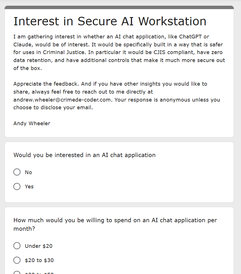
Final share today, with the news of an expert witness and their very embarrassing ChatGPT conversations coming to light, I opened up a survey to see if people are interested in an actual “safe” chat app that has zero data retention.

It used to be that if you paid for ChatGPT (or Claude), you could opt out of training. More recently, these companies have committed to retaining information for model safety, or because courts have told them they need to keep it. Mostly when calling the APIs directly, they are zero-data-retention by default (beyond a few minutes to keep the cache). So building a ZDR chat app is totally feasible.

See the survey I have opened up here, which asks if you are interested, price points, desktop/web-app, what you would use it for, etc. I do wonder if there will be more potential interest in state entities, since OpenAI and Anthropic are really dropping the ball here on whether people can trust them with sensitive information.

VerusCite: checking academic articles for hallucinations

I have a new app out, VerusCite. With the recent rise in popularity of GenAI tools like ChatGPT and Claude, this has also come along with academics writing slop articles.

One of the ways to check that slop is via looking at the articles citations. LLMs have some predictable failure modes in writing papers whole cloth – they tend to get details like complicated author lists wrong, or swap out incorrect journal titles. VerusCite is a tool for editors and reviewers to use to verify citations in a fast and cheap application.

It costs $2 to review a paper (and you get two free reviews on sign-up). If you want to see the output of a single example though, check out https://veruscite-data.com/share/E1-rn3TBwksENO_3hlmsRD0IG-EnXd6vfQg-upQZWQM

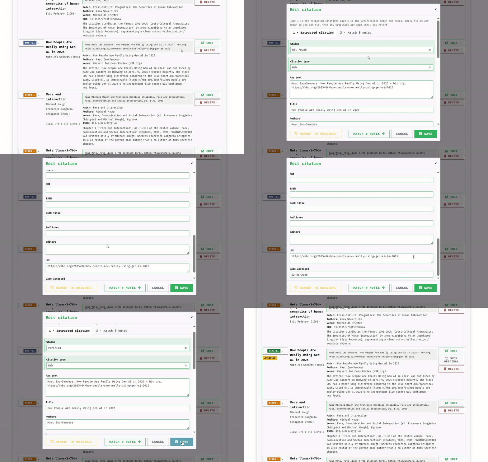
In addition to hallucinations, I have made many parts of the application just useful to editors in general. Many papers have minor errors in their bibliographies; typos, years off, author swaps, bad URLs, etc. Here is an example – no hallucinations that signal poor writing, but has seven different errors in the bibliography.

This is par for the course (it is quite possible 5% of citations have errors that look like this). The website has convenient tools to edit citations and export the fixed citations (whether minor errors or gross hallucinations) in various formats.

This makes much lighter work of the tedious job of formatting and checking citations for editors. One of the ways I think is critical to build generative AI tools is to consider the human in the loop from the start. My tool will ultimately make some errors (I error rate estimates in my public benchmark). I want it to be as fast for a human to confirm (or refute) the LLM label.

If you are an editor or a reviewer, I highly suggest you check the application out. Peer review journals (and pre-print servers that review the applications before posting), will need to use a tool like this as a first pass to ensure slop is not being posted.

Notes on document processing with LLMs

One of the recent papers that came across my X feed was a researcher digitizing a corpus of old Sears catalogs to estimate inflation more accurately:

The technical skills to do this work are closely related to many of the projects I am working on at Gainwell – large-scale document processing using LLMs. So if you are a PhD student and your thesis involves work like this, I would likely want to hire you for a six-figure job as a data scientist at Gainwell.

I wanted to have a quick blog post on some of the tools to process documents. So this researcher processed 180 Sears catalogs that are typically well over 1000 pages, so they likely dropped well over $10k on this project.

Like I said in the X post, for this type of volume processing, you shouldn’t be using the main models. You should first consider the cheaper models, like the flash-lite models from Gemini (not even the flash for this), or the mini/nano models from OpenAI. Using these cheaper models, which I suspect would be of similar accuracy, would reduce the cost to more like $2k in this project.

For those even more budget-conscious (I am processing this volume often daily at Gainwell for different projects), here are a few of my notes on open source models. (Also I am concerned OpenAI will entirely drop the mini/nano models in the future, hence I want to make sure I have plenty of options.)

OCR and Markdown

So this project used the images to help classify the information, but if you are dealing with pure text, a common approach is to first OCR the document, and then apply structured extraction from the text. This works well to save costs even if using served models, as we are talking about an image of a page being 10k tokens, but the extracted text often being well under 1k tokens.

In LLMs for Mortals, I show using the docling library to do this:

If the PDF is already OCRed (it has the underlying text) there are Python libraries to directly read the text. This example uses pypdf, but a better default library is pypdfium2 (it is much faster).

The difference between converting to Markdown vs. reading the text is that Markdown conversion will be a bit nicer in converting tables, graphs, and page chrome (e.g. footers/headers).

I have had good success with docling (which you can have it convert to Markdown with just the page text), but it does load in a PyTorch model (which adds a bit of latency). You can turn it off to only use the text in the PDF (and not the image), which does save time but still has a fair bit of latency.

If the PDF has the text embedded and you do not want a big model, I have been happy with the results of the liteparse library. This does not use an LLM at all to do the conversion to Markdown, so is quite fast.

Due to the increased cost, if you do need a served model, (sometimes you just have latency requirements and you don’t want to deal with your own server), Mistral OCR is worth checking out. This is a good cost-effective alternative if you are using AWS Textract and need things like table extraction.

There are many different models and providers coming out in the space (OvisOCR2 is one of the recent models for OCR, for served models the group that created liteparse (LlamaIndex) also has served model options).

Structured Extraction

OK, so now you have your pages in text that you can use. At this stage, you will want to extract out information. My go-to local model for named entity recognition (NER) is GLiNER, but the GLiNER2 library has examples that do the full structured extraction.

For a primer on the distinction between NER and structured extraction, pretend you had a free-text narrative “PA note: Vitals checked: HR 78 bpm, SpO₂ 98% on RA. Pt tolerated assessment well, no acute distress noted.”.

For NER, if you extracted vitals you would get back something like:

from gliner import GLiNER

# load GLiNER model
model = GLiNER.from_pretrained("urchade/gliner_small-v2")

# Physician Assistant narrative
narrative = """PA note: Vitals checked: HR 78 bpm, SpO₂ 98% on RA. 
Pt tolerated assessment well, no acute distress noted."""

# define entities to extract
labels = ["heart_rate","oxygen"]

# extract entities
entities = model.predict_entities(narrative, labels)
print(entities)

And this prints out:

[{'start': 25, 'end': 34, 'text': 'HR 78 bpm', 'label': 'heart_rate', 'score': 0.9038965106010437}, {'start': 36, 'end': 43, 'text': 'SpO 98%', 'label': 'oxygen', 'score': 0.8429999351501465}]

So it identifies the specific text. Structured extraction can actually identify additional information. So here I just say collect all vitals, and identify if the note is from a physician assistant or nurse.

from gliner2 import GLiNER2

# Load GLiNER2 model
extractor = GLiNER2.from_pretrained("fastino/gliner2-base-v1")

# Physician Assistant narrative
narrative = """PA note: Vitals checked: HR 78 bpm, SpO₂ 98% on RA. 
Pt tolerated assessment well, no acute distress noted."""

schema = {"clinical_note": [
            "clinician_role::[nurse|physician assistant]::str::Role of the healthcare professional",
            "vitals::list::Vital signs collected"
          ]}

# Define structured extraction schema
results = extractor.extract_json(narrative,schema)
print(results)

And this prints out:

{'clinical_note': [{'clinician_role': 'physician assistant', 'vitals': ['SpO 98% on RA', 'HR 78 bpm']}]}

So it filled in the clinician role without the actual words “physician assistant” being in the actual note (it smartly inferred that from the “PA note” part).

NER is actually one of the techniques that local models are really the only viable approach, but structured extraction is still a case where I default to the small frontier models. But small open source models are worth testing (these can easily be run on a CPU).

They are just different use cases. NER is good for redacting info and then forwarding to an LLM (see OpenAI’s model, although I have had good success using GLiNER for this exact use case as well). But most of the time I want actual structured extraction – so turning PDFs/images into actual data you can put into a table.

If you want to skip the OCR part entirely and just submit images, see the NuExtract model (and follow Gio’s work, he is often writing examples of these).

If you are using Databricks, it has similar structured extraction tasks compiled down to UDFs that are directly available in SQL. (Also FYI, Teradata has a similar option to take models as an ONNX or PMML file and create a UDF function.)

Advice

So I talked a lot; let’s try to recap in some simple advice.

  1. Do not use the main frontier models (e.g. Sonnet, Sol) to do document processing and extraction tasks. Should default to trying models like Gemini Flash-Lite and gpt-nano at first to see if they work. Frontier models are both more expensive and often not any better than the tinier models.

  2. If you do not need to extract info out of images, converting documents to text first (and maybe converting that text to markdown) is a way to make extraction cheaper/faster than using images directly. There are multiple local models that run reasonably fast on CPU that can do this.

  3. If you need NER or structured extraction, check out GLiNER2. I would still default to using the cheaper frontier models for this often. But if they are too expensive (or you are a cheap grad student), the local models may be totally sufficient.

I am often using the frontier models at work, as I have throughput requirements and I default to not running a server as much as I possibly can. For production APIs, the latency requirements are often hard.

But in the example you are a grad student and have a corpus of 30k pages you want to churn through, you can just have your laptop burn through them overnight for a week if you want to cut costs.

AI writing is better than no writing

AI disclosure – this post was entirely written by myself.

I know AI writing is still pretty cringey – so I get that people are quite opposed to it. For people like me though (academics promoting their work, more technical oriented) I would like to proffer a slight defense of (even cringey) AI writing. Having an LLM tool help you write a blog post is better than not writing at all.

I have come to the personal opinion I just want you to disclose when you use AI. I am starting to get peer review requests for academic papers that are clearly LLM written, and they are not obviously worse than the typical (mostly horrid) way academics write papers (they may actually be better to be honest). Blog and social media posts I think are strictly worse to my personal tastes when using LLM writing (across many dimensions, for now anyway). But it is better to write something than nothing if you have something worth saying.

Where this matters for technical folks (and academics) is that your default SEO is awful. Most academic papers are behind paywalls. LLM research tools are not picking up peer reviewed papers. So if you have something worth saying, having LLMs write out a blog post for you is worth it relative to having no writing at all.

For examples of LLM writing I have on this site:

And then my book, Large Language Models for Mortals: A Practical Guide for Analysts with Python, is around 50% AI generated.

None of these examples I would have finished without the help of AI; either entirely writing for the example blog posts, or writing the first draft in the case of the LLM book. (The LLM book is good by the way, you would not be able to tell I generated that first draft at all with Claude.)

My suggestion is to not let AI entirely take the wheel, but to create a detailed outline and have the LLM review your prior writing. Those two things improve posts by a wide margin (in addition to making sure AI is not too verbose – keep those blog posts simple!). And then you still need to take the time to review your own writing (for references you need to check those for hallucinations).

To be clear again, AI writing is better than nothing if you have something actually useful to say to the world. The bigger issue with AI writing are slop merchants just wasting space. That happened before with LLM tools, it is just much easier and more prevalent now. Just own it when you use AI to help you write.

How long to conduct your experiment: Talk at ASEBP

Upcoming at the American Society of Evidence Based Policing Conference, I have a talk Thursday morning (9:45-10:00), How long to conduct your experiment.

The talk goes over some of the simple metrics I have created to help plan how long to conduct your intervention. Such as how long to evaluate your hot spots intervention, or purchase to increase arrest rates, etc.

I have prepared a ton of different resources. The main one is a web-based application (a WASM-based app with R as the backend) where you can enter your inputs and generate a graph showing how precise your parameter estimates are:

The help page includes citations and additional materials, but here is a brief rundown:

  • I have the math details in this github repo, see the methodology.pdf. It also includes notes on how I used different LLM tools to produce the webpage and the method materials. Each of the applications allows you to download the R code used to generate the graphs and tables.

  • I have created a series of YouTube videos demonstrating the application (WDD, IRR, Proportion tests)

  • I have posted my slides for the ASEBP talk

See you all in DC at ASEBP in a few weeks!

xAI voice cloning API

xAI has just released an API to clone your voice. It is pretty simple, read a script, and then an API where you can have text to speech in that voice.

Here is the python code after you have cloned your voice.

import os
import requests
voice_id = os.environ['ANDY1_VOICE'] # my demo voice ID
text = '''this is a test demo of my voice. Be excited!
OK, how about a list of things; one, two, three.
Lets see where this takes us.'''
response = requests.post(
"https://api.x.ai/v1/tts",
headers={
"Authorization": f"Bearer {os.environ['XAI_API_KEY']}",
"Content-Type": "application/json",
},
json={
"text": llm_book,
"voice_id": voice_id,
"language": "en",
},
)
response.raise_for_status()
with open("AndyTest1.mp3", "wb") as f:
f.write(response.content)

I need to figure out my audio set up a bit better (my mic set up is probably not optimal and it produces some echo). But does a good job imitating my boring voice right out of the box!

And here is an example for longer speech from my intro to LLMs book:

# intro to llm book
llm_book = '''
Large language models (LLMs) are transforming how we work. Some of these examples include using LLMs to help write computer code, using LLMs to extract out information from irregular text sources, and creating chat-bots that can interact with various data sources and documents.
Most analysts, however, do not have any experience with these tools. This book is meant to be a general introduction to realistic examples of how individuals can use these tools; either in general software applications, or to help analysts write code to create software itself. Given the rapid pace of advancement in this area, a general introduction to help individuals who work in the knowledge economy understand the capabilities of these tools I believe is in order.
Here is a simple example of using an LLM API (*Application Programming Interface* -- just a standard way to send information and get information back on the web) using the anthropic library in python to extract key information from a free text crime narrative:
'''
response = requests.post(
"https://api.x.ai/v1/tts",
headers={
"Authorization": f"Bearer {os.environ['XAI_API_KEY']}",
"Content-Type": "application/json",
},
json={
"text": llm_book,
"voice_id": voice_id,
"language": "en",
},
)
response.raise_for_status()
with open("AndyTest_LLMIntro.mp3", "wb") as f:
f.write(response.content)

The LLM intro messed up *Application Programming Interface* section (start listening at 50 seconds in). But otherwise it is very nice.

For those worried about security, xAI did something smart here — you need to input text live into the API given their prompts. You cannot have a pre-recording audio input to do this. So cloning someone elses voice is pretty hard.

Costs are around $4 per million characters in the text to speech API. So say narrating my entire book should be under $10 I believe.

Took me a total of less than an hour to set up a voice, create the python code, and write this blog post!

Gathering interest in tech courses

Quick post this morning — I have a survey up gathering input on interest in short, technical courses.

Think 2-3 days, potentially in person/synchronous.

If you have taken a course with Paul Allison at Horizon’s, or an ICPSR summer course, those are similar examples. But, the main difference will be these courses are to prepare you for pursuing private sector roles.

These will be aimed at:

  • grad level social science students
  • current professors looking to pursue private sector roles
  • current data analysts looking to get into data science
  • undergrads with some more technical background

Survey lists potential courses (python for data analysis, intro to LLM APIs, SQL + Dashboards, using agent based tools for analysis), the course medium (in person vs video), price points.

If you are a university or organization interested in hosting such sessions for your students, let me know as well. Happy to chat to you about bringing this to your campus.

LinkedIn Premium Does Not Boost your Posts

One of my connections mentioned in a post on LinkedIn that since he turned off Premium, his posts have been getting less engagement. Since LinkedIn offers a month for free, and I have been trying to promote my recent book, I figured I would try my free month trial and see how many more views I could get. (Here I am not worried about Premium for applying to new jobs, it is possible it is totally worth it for that, I was not applying to jobs in this test so I do not know.)

Long story short, LinkedIn Premium does not appear to promote my material at all above the baseline.

Post Views

In a sample of 30 posts the month before I turned on Premium (turned on 3/24 in the evening, turned off 4/22 in the morning), my posts had an average of 3600 views (with a standard deviation of 7000, median 1400). Post-Premium, I had 23 posts, and the views were on average 2200 (SD 2900, median 900). Here is the full table of posts and links (Premium=1 means it was posted when my Premium subscription was turned on):

| Premium | Views | URL |
| ----:|----- :|:----- |
| 0    | 3659  | https://www.linkedin.com/posts/andrew-wheeler-46134849_llms-have-transformed-the-data-science-industry-activity-7426975341572984832-HGTA |
| 0    | 2526  | https://www.linkedin.com/posts/andrew-wheeler-46134849_no-guarantees-but-i-am-going-to-try-to-start-activity-7428418993553846272-vdjA    |
| 0    | 2290  | https://www.linkedin.com/posts/andrew-wheeler-46134849_much-of-the-hype-around-claude-code-is-having-activity-7428781380391567360-zkXr   |
| 0    | 545   | https://www.linkedin.com/posts/andrew-wheeler-46134849_one-of-the-benefits-of-my-epub-version-of-activity-7429143771109302272-_V6T       |
| 0    | 1454  | https://www.linkedin.com/posts/andrew-wheeler-46134849_claude-code-has-the-ability-to-create-hooks-activity-7429506167527088128-01Um     |
| 0    | 1326  | https://www.linkedin.com/posts/andrew-wheeler-46134849_one-of-the-prompting-flows-i-find-convenient-activity-7429868558794436609-SDgG    |
| 0    | 1278  | https://www.linkedin.com/posts/andrew-wheeler-46134849_one-of-the-main-focuses-in-the-book-is-not-activity-7430230940444057600-pqK-      |
| 0    | 5988  | https://www.linkedin.com/posts/andrew-wheeler-46134849_while-skills-in-claude-code-are-all-the-rage-activity-7430955707358818304-iqjb    |
| 0    | 1726  | https://www.linkedin.com/posts/andrew-wheeler-46134849_one-of-the-mistakes-i-see-with-agent-based-activity-7431318102212100096-rI_W      |
| 0    | 1172  | https://www.linkedin.com/posts/andrew-wheeler-46134849_from-my-experience-as-an-educator-when-presenting-activity-7431680485585580032-8h7B    |
| 0    | 1360  | https://www.linkedin.com/posts/andrew-wheeler-46134849_although-the-llm-tools-are-currently-focused-activity-7432042882770944000-AfAG    |
| 0    | 5304  | https://www.linkedin.com/posts/andrew-wheeler-46134849_when-i-was-a-professor-at-ut-dallas-i-sat-activity-7432405268874817536-qrAI       |
| 0    | 30732 | https://www.linkedin.com/posts/andrew-wheeler-46134849_i-know-a-few-stats-folks-in-my-network-that-activity-7432767666781679617-HXnk |
| 0    | 1003  | https://www.linkedin.com/posts/andrew-wheeler-46134849_claude-code-does-not-have-an-image-model-activity-7433492422111776768-2dqY        |
| 0    | 884   | https://www.linkedin.com/posts/andrew-wheeler-46134849_while-i-have-a-section-in-the-book-devoted-activity-7433854815862013952-FIl-      |
| 0    | 888   | https://www.linkedin.com/posts/andrew-wheeler-46134849_in-the-book-i-have-a-dedicated-chapter-on-activity-7434217215450681344-hk3E       |
| 0    | 1868  | https://www.linkedin.com/posts/andrew-wheeler-46134849_the-llm-book-is-compiled-using-quarto-so-activity-7434579595095580673-RHdx        |
| 0    | 807   | https://www.linkedin.com/posts/andrew-wheeler-46134849_llms-for-mortals-how-to-view-the-epub-activity-7434945455073169409-bNDu           |
| 0    | 1243  | https://www.linkedin.com/posts/andrew-wheeler-46134849_section-on-using-gliner-for-ner-activity-7435304382931513344-NPPC                 |
| 0    | 1745  | https://www.linkedin.com/posts/andrew-wheeler-46134849_my-first-book-data-science-for-crime-analysis-activity-7436029137695416320-aRmr   |
| 0    | 914   | https://www.linkedin.com/posts/andrew-wheeler-46134849_so-the-new-book-large-language-models-for-activity-7436376426100199424-1g8E       |
| 0    | 1593  | https://www.linkedin.com/posts/andrew-wheeler-46134849_agentic-coding-apps-like-claude-code-and-activity-7436738847054512128-qiXz        |
| 0    | 3415  | https://www.linkedin.com/posts/andrew-wheeler-46134849_many-people-are-turned-off-by-ai-writing-activity-7437101213717909504-QjOo        |
| 0    | 928   | https://www.linkedin.com/posts/andrew-wheeler-46134849_pretty-much-every-day-there-is-a-new-prompt-activity-7437463609401794560-50H-     |
| 0    | 2185  | https://www.linkedin.com/posts/andrew-wheeler-46134849_much-of-the-hype-around-skills-is-imo-people-activity-7437826000958337024-t6i3    |
| 0    | 800   | https://www.linkedin.com/posts/andrew-wheeler-46134849_one-of-the-benefits-of-my-llm-for-mortals-activity-7438550758763098112-hQUw |
| 0    | 870   | https://www.linkedin.com/posts/andrew-wheeler-46134849_large-language-models-for-mortals-preview-activity-7438913140639207424-tAli       |
| 0    | 1948  | https://www.linkedin.com/posts/andrew-wheeler-46134849_new-blog-post-using-claude-code-to-help-activity-7441087469388861440-TCKq         |
| 0    | 1160  | https://www.linkedin.com/posts/andrew-wheeler-46134849_given-all-the-rage-with-generative-ai-and-activity-7441449857480933377-uPFw       |
| 0    | 27842 | https://www.linkedin.com/posts/andrew-wheeler-46134849_stop-teaching-r-teach-python-when-i-was-activity-7441812266938826753-DywF         |
| 1    | 526   | https://www.linkedin.com/posts/andrew-wheeler-46134849_forecasting-the-future-is-difficult-especially-activity-7442537064803368960-qsVO  |
| 1    | 13096 | https://www.linkedin.com/posts/andrew-wheeler-46134849_when-using-llms-to-do-structured-data-extraction-activity-7442899426471407617-CpZz |
| 1    | 2394  | https://www.linkedin.com/posts/andrew-wheeler-46134849_ive-spoken-with-many-people-who-are-concerned-activity-7443039100477145090-v_3i   |
| 1    | 646   | https://www.linkedin.com/posts/andrew-wheeler-46134849_the-main-audience-my-book-large-language-activity-7443261810511757312-R2Jc        |
| 1    | 3030  | https://www.linkedin.com/posts/andrew-wheeler-46134849_for-the-folks-that-were-not-happy-with-my-activity-7443401497444409344-q38H       |
| 1    | 437   | https://www.linkedin.com/posts/andrew-wheeler-46134849_one-of-the-current-capabilities-of-googles-activity-7443624184120754176-YHbw      |
| 1    | 5275  | https://www.linkedin.com/posts/andrew-wheeler-46134849_one-error-i-am-seeing-devs-continually-make-activity-7443986571650973696-TZ-K     |
| 1    | 3815  | https://www.linkedin.com/posts/andrew-wheeler-46134849_one-of-the-biggest-issues-with-using-generative-activity-7444348969100664832-pX0v |
| 1    | 738   | https://www.linkedin.com/posts/andrew-wheeler-46134849_reports-of-rags-demise-are-overstated-activity-7444711358421491712-6BJu           |
| 1    | 425   | https://www.linkedin.com/posts/andrew-wheeler-46134849_the-recent-litellm-distribution-attack-highlights-activity-7445073747968999424-NEmn    |
| 1    | 3752  | https://www.linkedin.com/posts/andrew-wheeler-46134849_one-of-the-responses-to-me-writing-the-book-activity-7445436130080186369-7Fvx     |
| 1    | 1670  | https://www.linkedin.com/posts/andrew-wheeler-46134849_professors-that-follow-me-i-am-happy-to-activity-7446160904217407488-CXcZ         |
| 1    | 918   | https://www.linkedin.com/posts/andrew-wheeler-46134849_i-have-used-claude-code-the-longest-probably-activity-7447248077435920385-Ym8A    |
| 1    | 876   | https://www.linkedin.com/posts/andrew-wheeler-46134849_gio-has-a-new-post-out-on-examining-confidence-activity-7448697613513740289-hObZ  |
| 1    | 1959  | https://www.linkedin.com/posts/andrew-wheeler-46134849_the-mythos-technical-blog-post-on-its-cybersecurity-activity-7449059395071709184-UJOC  |
| 1    | 2201  | https://www.linkedin.com/posts/andrew-wheeler-46134849_for-folks-that-use-jupyter-notebooks-one-activity-7449422388691243008-Twxn        |
| 1    | 626   | https://www.linkedin.com/posts/andrew-wheeler-46134849_one-of-the-recommendations-i-have-in-the-activity-7450147165781426177-vceO        |
| 1    | 333   | https://www.linkedin.com/posts/andrew-wheeler-46134849_the-term-agent-is-almost-always-used-as-activity-7450509557677625344-42Ze         |
| 1    | 5787  | https://www.linkedin.com/posts/andrew-wheeler-46134849_agent-based-systems-require-bad-python-code-activity-7450871941458190336-gzSl     |
| 1    | 468   | https://www.linkedin.com/posts/andrew-wheeler-46134849_broadly-there-are-two-types-of-agent-based-activity-7451234329390678016-ZU1h      |
| 1    | 1267  | https://www.linkedin.com/posts/andrew-wheeler-46134849_i-get-periodically-asked-what-is-the-best-activity-7451596716354707456-aFMF       |
| 1    | 346   | https://www.linkedin.com/posts/andrew-wheeler-46134849_the-saying-a-picture-is-worth-a-1000-words-activity-7451959111132299264-Tk7o      |
| 1    | 480   | https://www.linkedin.com/posts/andrew-wheeler-46134849_it-is-important-to-have-independent-benchmark-activity-7452318150701953024-ftcM        |

I would have expected a multiplier (e.g. typically 3k views, now you have 6k or 9k views per post). So you could nitpick that I have differential timing for the posts, and the pre-premium posts have some contamination (if they promoted my older posts when I activated Premium). But those are not large enough to make a difference in my findings relative to what I expected.

The posts are quite comparable in content, mostly focused on my book and LLMs. It is possible my audience is oversaturated with that content, but I think it is just as likely that LinkedIn Premium doesn’t really promote your work to any substantive extent. (I have additionally obtained more followers in this period, so that should bias the results to have more views, not less.) At least here there is no evidence I should continue to pay $20 a month to increase my reach on LinkedIn.

Posts are bursty, and in the end I have very little ability to forecast what will or will not be popular. In the pre-period, my most popular post was on a blog post I did on log-probabilities (30k views). I definitely try to post more technical stuff on LinkedIn than the typical social media influencer, so that limits the reach.

I also had a rage-bait post on professors should teach python and not R with just under 30k views. (That was a bit of social media manipulation – have a controversial opinion that divides people, you get a bunch of thumbs up and a bunch of comments.) I do not have that many potential rage-bait post topics!

In addition to this, I also did the month for free for LinkedIn Premium for my business Crime De-Coder page. The same with my business page, I did not see any increased views, increased followers, etc.

Profile Views

Although I have not seen LinkedIn explicitly say Premium boosts your posts (besides actually paying for advertising), I have seen LinkedIn explicitly advertise that Premium profiles get more views:

So how do profile views look? I did get more the week I signed up, but it was trending upward previously, and reverted to the trend after week one anyway. (A few days short, I cannot access the chart week by week since turning off Premium.)

For a bit of background, I spent most of my time posting on my LinkedIn business Crime De-Coder page, and only posted on my personal page maybe once or twice a month. But since publishing LLMs for Mortals (in February of 2026), I have posted more on my personal. Which you can see increased my profile views before I signed up for Premium.

Likely the past additional profile views are for that rage-bait Python vs R post that was popular, not due to anything Premium did.

This appears to be extremely misleading advertising on LinkedIn’s part. If they just look at Premium vs not, it is likely Premium users are more active. This should just say the explicit “boost” profile views get, like ranked higher in searches.

$100 ad credit

With premium, you get $100 ad credit for posts a month. I used this to boost my original LLM for Mortals launch post, which was stale at that point and not accumulating any additional views.

The metrics on the post were as LinkedIn said they would be. Despite having 80+ likes when I first created it, the post only had 3700 views. Spending $100 on the credits got me an additional ~3500 views and supposedly ~50 additional website clicks. (I am confused how this is calculated, as I can see the actual link in the post was clicked fewer than 10 additional times with the campaign.)

I knew going in that adverts on LinkedIn are not a net benefit given my book purchase conversion rates. What I will call “high trust” referrals, I have something like a 1/100 purchase rate for the book. For other mediums, it is more like 1/1000. As far as I can tell, these seem pretty typical for a higher dollar value book purchase ($50+).

I have debated on setting the purchase price for the epub to much lower. $50 is in line with current offerings from O’Reilly, and in my informal demand curve tests is where I think it should be. But I don’t think any realistic conversion rate would make LinkedIn advertising make sense for my book.

For reference for influencers though, this gives a rough estimate comparable to LinkedIn’s direct advertising. Basically my average post is worth $100 according to LinkedIn. I only have around 3k followers currently on LinkedIn, so I imagine folks with followings 10x that can likely do direct advertisements to their audiences for more like $1k and up.

Wrap Up

I still think LinkedIn is the best social media site currently to promote my work and business. It is not just about the raw view counts, but also about conversion to people buying my book or reaching out for additional consulting gigs.

I will continue to use LinkedIn for this, but paying for a Premium LinkedIn account does not appear to be worth it for these reasons. Even if the views were increased, it is possible that they are not good connections for these end goals.

There are additional things you get with Premium (can send cold messages to people you are not connected to, supposedly higher priority when applying to jobs). Those are maybe worth the $20 a month for some people. But focusing on what LinkedIn advertises for “boosting” your posts and profile, I did not personally see any evidence that would justify spending even $1 a month for the Premium features.