An alt take on opioid treatment coverage in North Carolina

The Raleigh News & Observer has been running multiple stories on the recent Medicaid expansion in North Carolina, with one recently about expanded opioid treatment coverage. Myself and Kaden Call have worked in the past on developing an algorithm to identify underprovided estimates (see background blog post, and Kaden’s work at Gainwell while an intern).

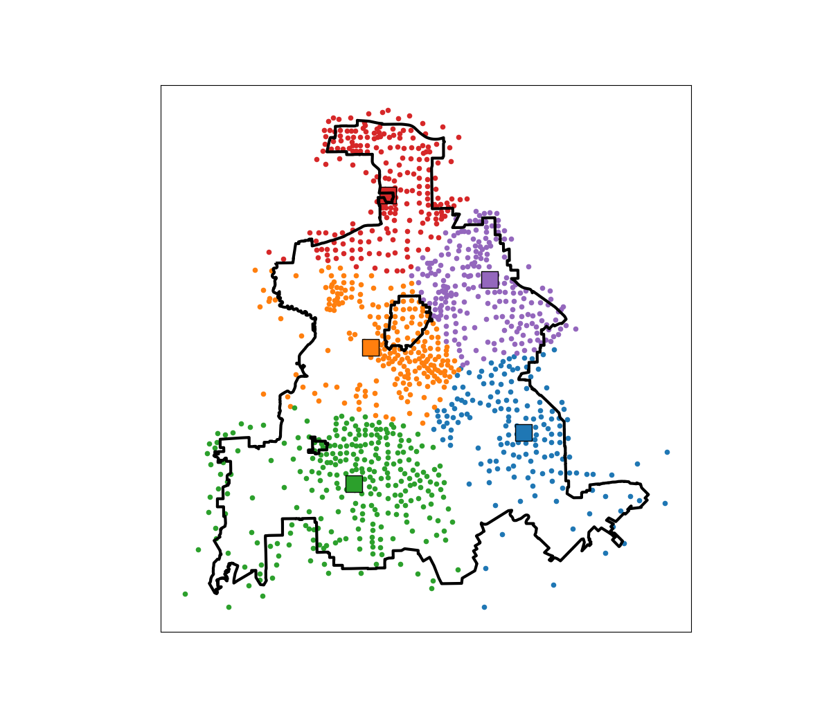
I figured I would run our algorithm through to see what North Carolina looks like. So here is an interactive map, with the top 10 zipcodes that have need for service (in red polygons), and CMS certified opioid treatment providers (in blue pins). (Below is a static image)

My initial impression was that this did not really jive with the quotes in the News & Observer article that suggested NC was a notorious service dessert – there are quite a few treatment providers across the state. So the cited Rural HealthInfo source disagrees with this. I cannot find their definition offhand, but I am assuming this is due to only counting in-patient treatment providers, whereas my list of CMS certified providers is mostly out-patient.

So although my algorithm identified various areas in the state that likely could use expanded services, this begs the question of whether NC is really a service dessert. It hinges on whether you think people need in-patient or out-patient treatment. Just a quick sampling of those providers, maybe half say they only take private, so it is possible (although not certain) that the recent Medicaid expansion will open up many treatment options to people who are dependent on opioids.

SAMHSA estimates that of those who get opioid treatment, around 5% get in-patient services. So maybe in the areas of high need I identify there is enough demand to justify opening new in-patient service centers – it is close though I am not sure the demand justifies opening more in-patient (as opposed to making it easier to access out-patient).

Asking folks with a medical background at work, it seems out-patient has proven to be as effective as in-patient, and that the biggest hurdle is to get people on buprenorphine/methadone/naltrexone (which the out-patient can do). So I am not as pessimistic as many of the health experts that are quoted in the News & Observer article.

Using linear programming to assess spatial access

So one of the problems I have been thinking about at work is assessing spatial access to providers. Some common metrics are ‘distance to nearest’, or combining distance as well as total provider capacity into one metric, the two-step floating catchment method (2SFCA).

So imagine we are trying to evaluate the coverage of opioid treatment facilities relative to the spatial distribution of people abusing opioids. Say for example we have two areas, A and B. Area A has a facility that can treat 50 people, but has a total of 100 people who need service. Now Area B has no treatment provider, but only has 10 people that need service.

If you looked at distance to nearest provider, location B would look worse than A. So you may think to yourself – we should open up a facility in Area B. But if you look at the total number of people, as well as the capacity of the treatment provider in Area A, it would probably be a better investment to expand the capacity of treatment center A. It has more potential demand.

The 2SFCA partially captures this, but I am going to show a linear programming approach that can decompose the added benefit of adding capacity to a particular provider, or adding in potential new providers. I have the posted these functions on github, but can walk through the linear programming model, and how to assess potential policy interventions in that framework.

So first lets make just a simple set of data, we have 10 people with XY coordinates, and 2 service providers. The two service providers have capacity 3 and 5, so we cannot cover 2 of the people.

# Python example code
import numpy as np
import pandas as pd
import pulp

# locations of people
id = range(10)
px = [1,1,3,3,4,5,6,6,9,9]
py = [2,8,1,8,4,6,1,2,5,8]
peop = pd.DataFrame(zip(id,px,py),columns=['id','px','py'])

# locations of 2 providers & capacity 3/5
hid = [1,2]
hx = [1,8]
hy = [1,8]
hc = [3,5] # so cant cover 2 people
prov = pd.DataFrame(zip(hid,hx,hy,hc),columns=['hid','hx','hy','hc'])

Now for the subsequent model I show, it is going to assign the people to the nearest possible provider, given the distance constraints. To make the model feasible, we need to add in a slack provider that can soak up the remaining people not covered. We set this location to somewhere very far away, so the model will only assign people to this slack provider in the case no other options are available.

# add in a slack location to the providers
# very out of the way and large capacity
prov_slack = prov.iloc[[0],:].copy()
prov_slack['hid'] = 999
prov_slack['hx'] = 999
prov_slack['hy'] = 999
prov_slack['hc'] = peop.shape[0]
prov_add = pd.concat([prov,prov_slack],axis=0)

Now the decision model looks at all pairwise combinations between people and providers (potentially eliminating combinations that are too far away to be reasonable). So I do the cross join between the people/providers, and then calculate the Euclidean distance between them. I set the distance for the slack provider to a very high value (here 9999).

# distance between people/providers
peop['const'] = 1
prov_add['const'] = 1
cross = pd.merge(peop,prov_add,on='const')
cross['dist'] = np.sqrt( (cross['px']-cross['hx'])**2 + 
                         (cross['py']-cross['hy'])**2 )
cross.set_index(['id','hid'],inplace=True)
# setting max distance for outside provider to 9999
cross.loc[cross.xs(999,level="hid",drop_level=False).index,"dist"] = 9999

Now we are ready to fit our linear programming model. First our objective is to minimize distances. (If all inputs are integers, you can use continuous decision variables and it will still return integer solutions.)

# now setting up linear program
# each person assigned to a location
# locations have capacity
# minimize distance traveled

# Minimize distances
P = pulp.LpProblem("MinDist",pulp.LpMinimize)

# each pair gets a decision variable
D = pulp.LpVariable.dicts("DA",cross.index.tolist(),
                          lowBound=0, upBound=1, cat=pulp.LpContinuous)

# Objective function based on distance
P += pulp.lpSum(D[i]*cross.loc[i,'dist'] for i in cross.index)

And we have two types of constraints, one is that each person is assigned a single provider in the end:

# Each person assigned to a single provider
for p in peop['id']:
    provl = cross.xs(p,0,drop_level=False).index
    P += pulp.lpSum(D[i] for i in provl) == 1, f"pers_{p}"

As a note later on, I will expand this model to include multiple people from a single source (e.g. count of people in a zipcode). For that expanded model, this constraint turns into pulp.lpSum(...) == tot where tot is the total people in a single area.

The second constraint is that providers have a capacity limit.

# Each provider capacity constraint
for h in prov_add['hid']:
    peopl = cross.xs(h,level=1,drop_level=False)
    pid = peopl.index
    cap = peopl['hc'].iloc[0] # should be a constant
    P += pulp.lpSum(D[i] for i in pid) <= cap, f"prov_{h}"

Now we can solve the model, and look at who was assigned to where:

# Solve the model
P.solve(pulp.PULP_CBC_CMD()) 
# CPLEX or CBC only ones I know of that return shadow
pulp.value(P.objective) #print objective 20024.33502494309


# Get the person distances
res_pick = []
for ph in cross.index:
    res_pick.append(D[ph].varValue)

cross['picked'] = res_pick
cross[cross['picked'] > 0.99]

So we can see two people were assigned the slack provider 999. Note that some people are not even assigned the closest – person 7 (6,2) is assigned to provider 2 at a distance of 6.3, it is only a distance of 5.1 away from provider 1. Because provider 1 has limited capacity though, they are assigned to provider 2 in the end.

In this framework, we can get the shadow price for the constraints, which says if we relax the constraint, how much it will improve our objective value.So if we add 1 capacity to provider 1, we will improve our objective by -9994.

# Get the shadow constraints per provider
o = [{'name':name, 'shadow price':c.pi, 'slack': c.slack} 
     for name, c in P.constraints.items()]
sc = pd.DataFrame(o)
print(sc)

I have helper functions at the github link above, so I don’t need to go through all of these motions again. You input your people matrix and the field names for the id, x, y, totn values.

And then you input your provider matrix with the field names for the providerid, x, y, prov_capacity (note this is not the matrix with the additional slack provider, my code adds that in automatically). The final two arguments limit the potential locations (e.g. here saying can’t assign a person to a provider over 12 distance away). And the last argument sets the super high distance penalty to people are not assigned.

# load in model functions
from assign_funcs import ProvAssign

# Const=1 is the total people per area
m1 = ProvAssign(peop,
                ['id','px','py','const'],
                prov,
                ['hid','hx','hy','hc'],
                12,
                9999)

m1.solve(pulp.PULP_CBC_CMD())
# see the same objective as before

Now we can go ahead and up our capacity at provider 1 by 1, and see how the objective is reduced by -9994:

# if we up the provider capacity for
# prov by 1, the model objective goes 
# down by -9994
prov['hc'] = [4,5]

m2 = ProvAssign(peop,
                ['id','px','py','const'],
                prov,
                ['hid','hx','hy','hc'],
                12,
                9999)
m2.solve(pulp.PULP_CBC_CMD())
m1.obj - m2.obj # 9994!

Like I said, I extended this to the scenario that you don’t have individual people, but have multiple counts of people in a spatial area. What can happen in this scenario is one source location can send people to multiple providers. Here you can see that source location 4 (total of 12 people), 5 were sent to provider 1, and 7 were sent to provider 2.

# Can make these multiple people, 100 total
peop['tot'] = [10,15,5,10,12,11,20,6,9,2]
prov['cap'] = [40,50] # should assign 10 people to slack

m3 = ProvAssign(peop,
                ['id','px','py','tot'],
                prov,
                ['hid','hx','hy','cap'],
                12,
                9999)
m3.solve(pulp.PULP_CBC_CMD())
# Can see the assignments from one
# source can spill over into multiple
# provider locations
m3.assign

So one of the things I like about this approach I already showed, we can do hypothetical scenarios ‘add capacity’ and see how it improves overall travel. Another potential intervention is to just place dummy 0 capacity providers over the study area, then look at the shadow constraints to see the best locations to open new facilities. Here I add in a potential provider at location (5,5).

# Can add in hypothetical providers with
# no capacity (make new providers)
# and check out the shadow
p2 = prov_slack.copy()
p2['hid'] = 10
p2['hx'] = 5
p2['hy'] = 5
p2['hc'] = 0
p2['cap'] = 0
prov_add = pd.concat([prov,p2],axis=0)


m4 = ProvAssign(peop,
                ['id','px','py','tot'],
                prov_add,
                ['hid','hx','hy','cap'],
                10,
                9999)

# we now don't have source9 and prov1
m4.cross

Here in the code, I also have a function to limit potential assignments. Here if I set that limit to 10, it only just prevents id 9 (9,8) from being assigned to provider 1 (1,1), which is a distance of 10.6 away. This is useful with larger datasets, in which you may not be able to fit all of the pairwise distances into memory and model. (Although this model is pretty simple, you may be able to look at +1 million pairwise combos and solve in a reasonable time with open source solvers.)

Now we can go ahead and solve this model. I have a bunch of helper functions as well, so after solving we can check out the shadow price matrix:

# Solve m4 model
m4.solve(pulp.PULP_CBC_CMD())

# can see the new provider 10
# if we added capacity would
# decrease distance travelled by -9996.2426
m4.shadow

And based on this, it does look like we will have the best improvement by adding capacity at our hypothetical new provider 10, as oppossed to adding capacity at provider 1 or 2. Lets see what happens if you add 10 capacity to our hypothetical provider:

# Now lets add capacity for new provider
# by 10, should the objective go down
# by 10*-9996.2426 ?
prov_add['cap'] = [40,50,10]

m5 = ProvAssign(peop,
                ['id','px','py','tot'],
                prov_add,
                ['hid','hx','hy','cap'],
                12,
                9999)
m5.solve(pulp.PULP_CBC_CMD())

# Not quite -9996.2 but close!
(m5.obj - m4.obj)/10

We can see that the objective was not quite reduced by the expected, but is close. If it is not feasible to add a totally new provider, but simpler to give resources to expand current ones, we can see what will happen if we expand provider 1 by 10.

# we could add capacity
# to provider 1 by 10
# as well
prov_add['cap'] = [50,50,0]

m6 = ProvAssign(peop,
                ['id','px','py','tot'],
                prov_add,
                ['hid','hx','hy','cap'],
                10,
                9999)
m6.solve(pulp.PULP_CBC_CMD())

# Not quite -9993.4 but close!
(m6.obj - m4.obj)/10

In addition to doing different policy interventions in this approach, I provide different metrics to assess distance traveled and coverage. So going back to model 4, we can look at which areas have limited coverage. It only ends up that source area 1 has 10/15 people not covered. The rest of the areas are covered.

# Can look at sources and see stats
# for distance travelled as well
# as potential non-coverage
m4.source_stats

The fields are Trav is the average distance travelled for people who are covered (so could have high coverage but those people have to go a ways). Tot is the total number of people within that particular source area, and picked/not-covered are those assigned a provider/not assigned a provider (so go to the slack) respectively.

I additionally I have stats available rolled up to providers, mostly based on the not covered nearby. One way that the shadow doesn’t work, if you only have 10 people nearby, it doesn’t make sense to expand capacity to any more than 10 people. Here you can see the shadow price, as well as those not covered that are nearby to that provider.

# Can look at providers
# and see which ones would result in
# most reduced travel given increased coverage
# Want high NotCover and low shadow price
m4.prov_stats

The other fields, hc is the listed capacity. Trav is the total travel for those not covered. The last field bisqw, is a way to only partially count not covered based on distance. It uses the bi-square kernel weight, based on the max distance field you provided in the model object. So if many people are nearby it will get a higher weight.

Here good add capacity locations are those with low shadow prices, and high notcovered/bisqw fields.

Note these won’t per se give the best potential places to add capacity. It may be the best new solution is to spread out new capacity – so here instead of adding 10 to a single provider, add a few to different providers.

You could technically figure that out by slicing out those leftover people in the m4.source_stats that have some not covered, adding in extra capacity to each provider, and then rerunning the algorithm and seeing where they end up.

Again I like this approach as it lets you articulate different policy proposals and see how that changes the coverage/distance travelled. Although no doubt there are other ways to formulate the problem that may make sense, such as maximizing coverage or making a coverage/distance bi-objective function.

Optimal and Fair Spatial Siting

A bit of a belated MLK day post. Much of the popular news on predictive or machine learning algorithms has a negative connotation, often that they are racially biased. I tend to think about algorithms though in almost the exact opposite way – we can adjust them to suit our objectives. We just need to articulate what exactly we mean by fair. This goes for predictive policing (Circo & Wheeler, 2021; Liberatore et al., 2021; Mohler et al., 2018; Wheeler, 2020) as much as it does for any application.

I have been reading a bit about spatial fairness in siting health resources recently, one example is the Urban Institutes Equity Data tool. For this tool, you put in where your resources are currently located, and it tells you whether those locations are located in areas that have demographic breakdowns like the overall city. So this uses the container approach (not distance to the resources), which distance traveled to resources is probably a more typical way to evaluate fair spatial access to resources (Hassler & Ceccato, 2021; Koschinsky et al., 2021).

Here what I am going to show is instead of ex-ante saying whether the siting of resources is fair, I construct an integer linear program to site resources in a way we define to be fair. So imagine that we are siting 3 different locations to do rapid Covid testing around a city. Well, we do the typical optimization and minimize the distance traveled for everyone in the city on average to those 3 locations – on average 2 miles. But then we see that white people on average travel 1.9 miles, and minorities travel 2.2 miles. So it that does not seem so fair does it.

I created an integer linear program to take this difference into account, so instead of minimizing average distance, it minimizes:

White_distance + Minority_distance + |White_distance - Minority_distance|

So in our example above, if we had a solution that was white travel 2.1 and minority 2.1, this would be a lower objective value than (4.2), than the original minimize overall travel (1.9 + 2.2 + 0.3 = 4.4). So this gives each minority groups equal weight, as well as penalizes if one group (either whites or minorities) has much larger differences.

I am not going to go into all the details. I have python code that has the functions (it is very similar to my P-median model, Wheeler, 2018). The codes shows an example of siting 5 locations in Dallas (and uses census block group centroids for the demographic data). Here is a map of the results (it has points outside of the city, since block groups don’t perfectly line up with the city boundaries).

In this example, if we choose 5 locations in the city to minimize the overall distance, the average travel is just shy of 3.5 miles. The average travel for white people (not including Hispanics) is 3.25 miles, and for minorities is 3.6 miles. When I use my fair algorithm, the white average distance is 3.5 miles, and the minority average distance is 3.6 miles (minority on average travels under 200 more feet on average than white).

So this is ultimately a trade off – it ends up pushing up the average distance a white person will travel, and only slightly pushes down the minority travel, to balance the overall distances between the two groups. It is often the case though that one can be somewhat more fair, but in only results in slight trade-offs though in the overall objective function (Rodolfa et al., 2021). So that trade off is probably worth it here.

References

Health Insurance Claims Data via HMS Data Sharing for Researchers

I have been sharing this with a bunch of people recently so figured it would be appropriate to share on the blog. My company, HMS, which audits health insurance claims has a data sharing agreement for researchers.

So this provides access to micro level Medicaid health insurance claims for a set of states. It includes 10 states currently:

It provides a limited set of person level info, provider level info (e.g. the hospital location of the claim), as well as all the info that comes with the insurance claim itself. Mostly folks will be interested in ICD codes associated with the claim I imagine, as well as maybe the CPT codes. (CPT are for particular procedures, whereas ICD are more like broader diagnoses for the overall visit.)

It is only criminology adjacent, and is tough because the coverage is limited to Medicaid for some research designs. But examples criminology folks may be interested in are say you could look for domestic violence ICD codes, or look at provider level behavior for opioid prescriptions, or mental health treatment claims, etc.

One of the things with criminology research is it is very hard to identify the costs of crime. Looking at victimization costs via health insurance claims may be an underestimate, but has a pretty clear societal cost. And the limited coverage to Medicaid will make cost estimates on the low side (although more directly relevant to the state, and among the most vulnerable population).

Geocoding the CMS NPI Registry (python)

So previously I wrote out creating service deserts. I have since found a nicer data source to use for this, the NPI CMS registry. This data file has over 6 million service providers across the US.

Here I will provide an example of using that data to geocode all the pharmacy’s in Texas, again using the census geocoding API and python.

Chunking up the NPI database

So first, you can again download the entire NPI database from here. So I have already downloaded and unzipped that file, which contains a CSV for the January version, named npidata_pfile_20050523-20210110.csv. So as some upfront, here are the libraries I will be using, and I also set the directory to where my data is located.

###############################
import pandas as pd
import numpy as np
import censusgeocode as cg
import time
from datetime import datetime
import os
os.chdir(r'D:\HospitalData\NPPES_Data_Dissemination_January_2021')
###############################

The file is just a bit too big for me to fit in memory on my machine. On Windows, you can use Get-Content npidata_pfile_20050523-20210110.csv | Measure-Object -Line in powershell to get the line counts, or on Unix use wc -l *.csv for example. So I know the file is not quite 6.7 million rows.

So what I do here is create a function to read in the csv file in chunks, only select the columns and rows that I want, and then return that data frame. In the end, you need to search across all of the Taxonomy codes to pull out the type of service provider you want. So for community pharmacies, the code is 3336C0003X, but it is not always in the first Taxonomy slot (some CVS’s have it in the second slot for example). You can see the big list of taxonomy codes here, so my criminology friends may say be interested in mental health or substance abuse service providers for other examples.

In addition to the taxonomy code, I always select organizations, not individuals (Entity Type = 2). And then I only select out pharmacies in Texas (although I bet you could fit all of the US pharmacies in memory pretty easily, maybe 60k in total?) Caveat emptor, I am not 100% sure how to use the deactivation codes properly in this database, as that data is always NaN for Texas pharmacies.

######################################################################
# Prepping the input data in chunks

keep_col = ['NPI','Entity Type Code','Provider Organization Name (Legal Business Name)',
            'NPI Deactivation Reason Code','NPI Deactivation Date','NPI Reactivation Date',
            'Provider First Line Business Practice Location Address',
            'Provider Business Practice Location Address City Name',
            'Provider Business Practice Location Address State Name',
            'Provider Business Practice Location Address Postal Code']
            
taxon_codes = ['Healthcare Provider Taxonomy Code_' + str(i+1) for i in range(15)]
keep_col += taxon_codes
community_pharm = '3336C0003X'
npi_csv = 'npidata_pfile_20050523-20210110.csv' #Newer files will prob change the name

# This defines the rows I want
def sub_rows(data):
    ec = data['Entity Type Code'] == "2"
    st = data['Provider Business Practice Location Address State Name'] == 'TX'
    ta = (data[taxon_codes] == community_pharm).any(axis=1)
    #ac = data['NPI Deactivation Reason Code'].isna()
    all_together = ec & st & ta #& ac
    sub = data[all_together]
    return sub

def csv_chunks(file,chunk_size,keep_cols,row_sub):
    # First lets get the header and figure out the column indices
    header_fields = list(pd.read_csv(npi_csv, nrows=1))
    header_locs = [header_fields.index(i) for i in keep_cols]
    # Now reading in a chunk of data
    skip = 1
    it_n = 0
    sub_n = 0
    ret_chunk = chunk_size
    fin_li_dat = []
    while ret_chunk == chunk_size:
        file_chunk = pd.read_csv(file, usecols=header_locs, skiprows=skip, 
                     nrows=chunk_size, names=header_fields, dtype='str')
        sub_dat = row_sub(file_chunk)
        fin_li_dat.append( sub_dat.copy() )
        skip += chunk_size
        it_n += 1
        sub_n += sub_dat.shape[0]
        print(f'Grabbed iter {it_n} total sub n so far {sub_n}')
        ret_chunk = file_chunk.shape[0]
    fin_dat = pd.concat(fin_li_dat, axis=0)
    return fin_dat


# Takes about 3 minutes
print( datetime.now() )
pharm_tx = csv_chunks(npi_csv, chunk_size=1000000, keep_cols=keep_col, row_sub=sub_rows)
print( datetime.now() )

# No deactivated codes in all of Texas
print( pharm_tx['NPI Deactivation Reason Code'].value_counts() )
######################################################################

So this ends up returning not quite 6800 pharmacies in all of Texas.

Geocoding using the census API

So first, the address data is pretty well formatted. But for those new to geocoding, if you have end parts of address strings like Apt 21 or Suite C, those endings will typically throw geocoders off the mark. So in just a few minutes, I noted the different strings that marked the parts of the addresses I should chop off, and wrote a function to clean those up. Besides that I just limit the zip code to 5 digits, as that field is a mix of 5 and 9 digit zipcodes.

######################################################################
# Now prepping the data for geocoding

ph_tx = pharm_tx.drop(columns=taxon_codes).reset_index(drop=True)

#['Provider First Line Business Practice Location Address', 'Provider Business Practice Location Address City Name', 'Provider Business Practice Location Address State Name', 'Provider Business Practice Location Address Postal Code']

# I just looked through the files and saw that after these strings are not needed
end_str = [' STE', ' SUITE', ' BLDG', ' TOWER', ', #', ' UNIT',
           ' APT', ' BUILDING',',', '#']

 
def clean_add(address):
    add_new = address.upper()
    for su in end_str:
        sf = address.find(su)
        if sf > -1:
            add_new = add_new[0:sf]
    add_new = add_new.replace('.','')
    add_new = add_new.strip()
    return add_new

# Some examples
clean_add('5700 S GESSNER DR STE G')
clean_add('10701-B WEST BELFORT SUITE 170')
clean_add('100 EAST UNIVERSITY BLVD.')
clean_add('5800 BELLAIRE BLVD BLDG 1')
clean_add('2434 N I-35 # S')

ph_tx['Zip5'] = ph_tx['Provider Business Practice Location Address Postal Code'].str[0:5]
ph_tx['Address'] = ph_tx['Provider First Line Business Practice Location Address'].apply(clean_add)
ph_tx.rename(columns={'Provider Business Practice Location Address City Name':'City',
                      'Provider Business Practice Location Address State Name':'State2'},
             inplace=True)
######################################################################

Next is my function to use the batch geocoding in the census api. Note the census api is a bit finicky – technically the census api says you can do batches of up to 5k rows, but I tend to get kicked off for higher values. So here I have a function that chunks it up into tinier batch portions and submits to the API. (A better function would cache intermediate results and wrap all that jazz in a try function.)

 ######################################################################
 #This function breaks up the input data frame into chunks
 #For the census geocoding api
 def split_geo(df, add, city, state, zipcode, chunk_size=500):
     df_new = df.copy()
     df_new.reset_index(inplace=True)
     splits = np.ceil( df.shape[0]/chunk_size)
     chunk_li = np.array_split(df_new['index'], splits)
     res_li = []
     pick_fi = []
     for i,c in enumerate(chunk_li):
         # Grab data, export to csv
         sub_data = df_new.loc[c, ['index',add,city,state,zipcode]]
         sub_data.to_csv('temp_geo.csv',header=False,index=False)
         # Geo the results and turn back into df
         print(f'Geocoding round {int(i)+1} of {int(splits)}, {datetime.now()}')
         result = cg.addressbatch('temp_geo.csv') #should try/except?
         # May want to dump the intermediate results
         #pi_str = f'pickres_{int(i)}.p'
         #pickle.dump( favorite_color, open( pi_str, "wb" ) )
         #pick_fi.append(pi_str.copy())
         names = list(result[0].keys())
         res_zl = []
         for r in result:
             res_zl.append( list(r.values()) )
         res_df = pd.DataFrame(res_zl, columns=names)
         res_li.append( res_df.copy() )
         time.sleep(10) #sleep 10 seconds to not get cutoff from request
     final_df = pd.concat(res_li)
     final_df.rename(columns={'id':'row'}, inplace=True)
     final_df.reset_index(inplace=True, drop=True)
     # Clean up csv file
     os.remove('temp_geo.csv')
     return final_df
 ######################################################################

And now we are onto the final stage, actually running the geocoding function, and piping the end results to a csv file. (Which you can see the final version here.)

######################################################################
# Geocoding the data in chunks

# Takes around 35 minutes
geo_pharm = split_geo(ph_tx, add='Address', city='City', state='State2', zipcode='Zip5', chunk_size=100)

#What is the geocoding hit rate?
print( geo_pharm['match'].value_counts() )
# Only around 65%

# Now merging back with the original data if you want
# Not quite sorted how I need them
geo_pharm['rowN'] = geo_pharm['row'].astype(int)
gp2 = geo_pharm.sort_values(by='rowN').reset_index(drop=True)

# Fields I want
kg = ['address','match','lat','lon']
kd = ['NPI',
      'Provider Organization Name (Legal Business Name)',
      'Provider First Line Business Practice Location Address',
      'Address','City','State2','Zip5']

final_pharm = pd.concat( [ph_tx[kd], gp2[kg]], axis=1 )

final_pharm.to_csv('Pharmacies_Texas.csv',index=False)
######################################################################

Unfortunately the geocoding hit rate is pretty disappointing, only around 65% in this sample. So if I were using this for a project, I would likely do a round of geocoding using the Google API (which is a bit more unforgiving for varied addresses), or perhaps build my own openstreet map geocoder for the US. (Or in general if you don’t have too many to review, doing it interactively in ArcGIS is very nice as well if you have access to Arc.)

Buffers and hospital deserts with geopandas

Just a quick blog post today. As a bit of a side project at work I have been looking into medical service provider deserts. Most people simply use a geographic cutoff of say 1 mile (see Wissah et al., 2020 for example for Pharmacy deserts). Also for CJ folks, John Hipp has done some related work for parolees being nearby service providers (Hipp et al., 2009; 2011), measuring nearby as 2 miles.

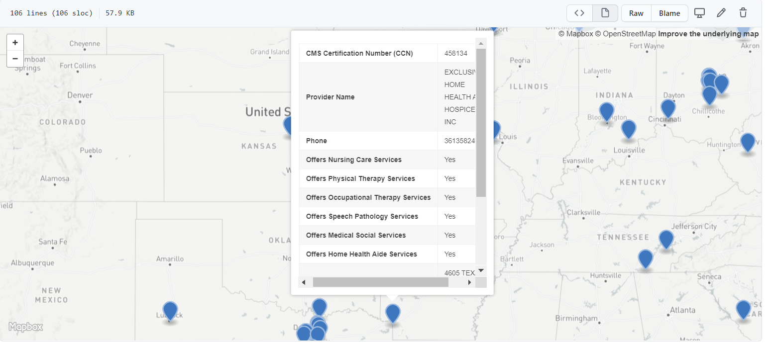
So I wrote some code to calculate nice sequential buffer areas and dissolve them in geopandas. Files and code to showcase are here on GitHub. First, as an example dataset, I geocode (using the census geocoding API) CMS certified Home Healthcare facilities, so these are hospice facilities. To see a map of those facilities across the US, and you can click on the button to get info, go to here, CMS HOME FACILITY MAP. Below is a screenshot:

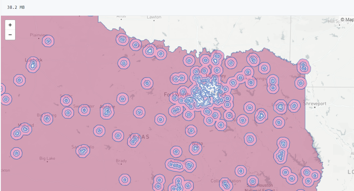
Next I then generate sequential buffers in kilometers of 2, 4, 8, 16, and then the leftover (just for Texas). So you can then zoom in and darker areas are at a higher risk of not having a hospice facility nearby. HOSPICE DESERT MAP

Plotting some of these in Folium were giving me fits, so I will need to familiarize myself with that more in the future. The buffers for the full US as well were giving me trouble (these just for Texas result in fairly large files, surprised Github doesn’t yell at me for them being too big).

Going forward, what I want to do is instead of relying on a fixed function of distance, is to fit a model to identify individuals probability of going to the doctor based on distance. So instead of just saying 1+ mile and you are at high risk, fit a function that defines that distance based on behavioral data (maybe using insurance claims). Also I think the distances matter quite a bit for urban/rural and car/no-car. So rural folks traveling a mile is not a big deal, since you need a car to really do anything in rural areas. But for folks in the city relying on public transportation going a mile or two is a bigger deal.

The model then would be similar to the work I did with Gio on gunshot death risk (Circo & Wheeler, 2020), although I imagine the model would spatially vary (so maybe geographically weighted regression may work out well).

References