Estimating Criminal Lifetime Value

At work I am currently working on estimating/forecasting healthcare spending. Similar to work I have done on forecasting person level crime risks (Wheeler et al., 2019), I build the predictive model dataset like this:

CrimeYear2020 PriorCrimeA PriorCrimeB
     0              2          3
     1              5          0
     0              0          0

etc. So I flatten people to a single row, and as covariates include prior cumulative crime histories. Most people do this similarly in the healthcare setting, so it looks like:

SpendingYear2020 PriorComorbidA PriorComorbidB
     3000              1          2
      500              3          0
    10000              0          0

Or sometimes people do a longitudinal dataset, where it is a spending*year*person panel (see Lauffenburger et al., 2020 for an example). I find this approach annoying for a few reasons though. One, it requires arbitrary temporal binning, which is somewhat problematic in these transaction level databases. We are talking for chronic offenders a few crimes per year is quite high, and ditto in the healthcare setting a few procedures a year can be very costly. So there is not much data to estimate the underlying function over time.

A second aspect I think is bad is that it doesn’t take into account the recency of the patterns. So the variables on the right hand side can be very old or very new. And with transaction level databases it is somewhat difficult to define how to estimate the lookback – do you consider it normalized by time? The VOID paper I mentioned we evaluated the long term scores, but the PD that does that chronic offender system has two scores – one a cumulative history and another a 90 day history to attempt to deal with that issue (again ad-hoc).

One approach to this issue from marketing research I have seen from very similar types of transactions databases are models to estimate Customer Lifetime Value (Fader et al. 2005). These models in the end generate a dataset that looks like this:

Person    RecentMonths  TotalEvents AveragePurchase
  A            3             5            $50
  B            1             2           $100
  C            9             8            $25

TotalEvents should be straightforward, RecentMonths just is a measure of the time since the last purchase, and then you have the average value of the purchases. And using just this data, estimates the probability of any future purchases, as well as projects the total value of the future average purchases. So here I use an example of this approach, using the Wolfgang Philly cohort public data. I am not going into the model more specifically (read some of the Bruce Hardie notes to get a flavor).

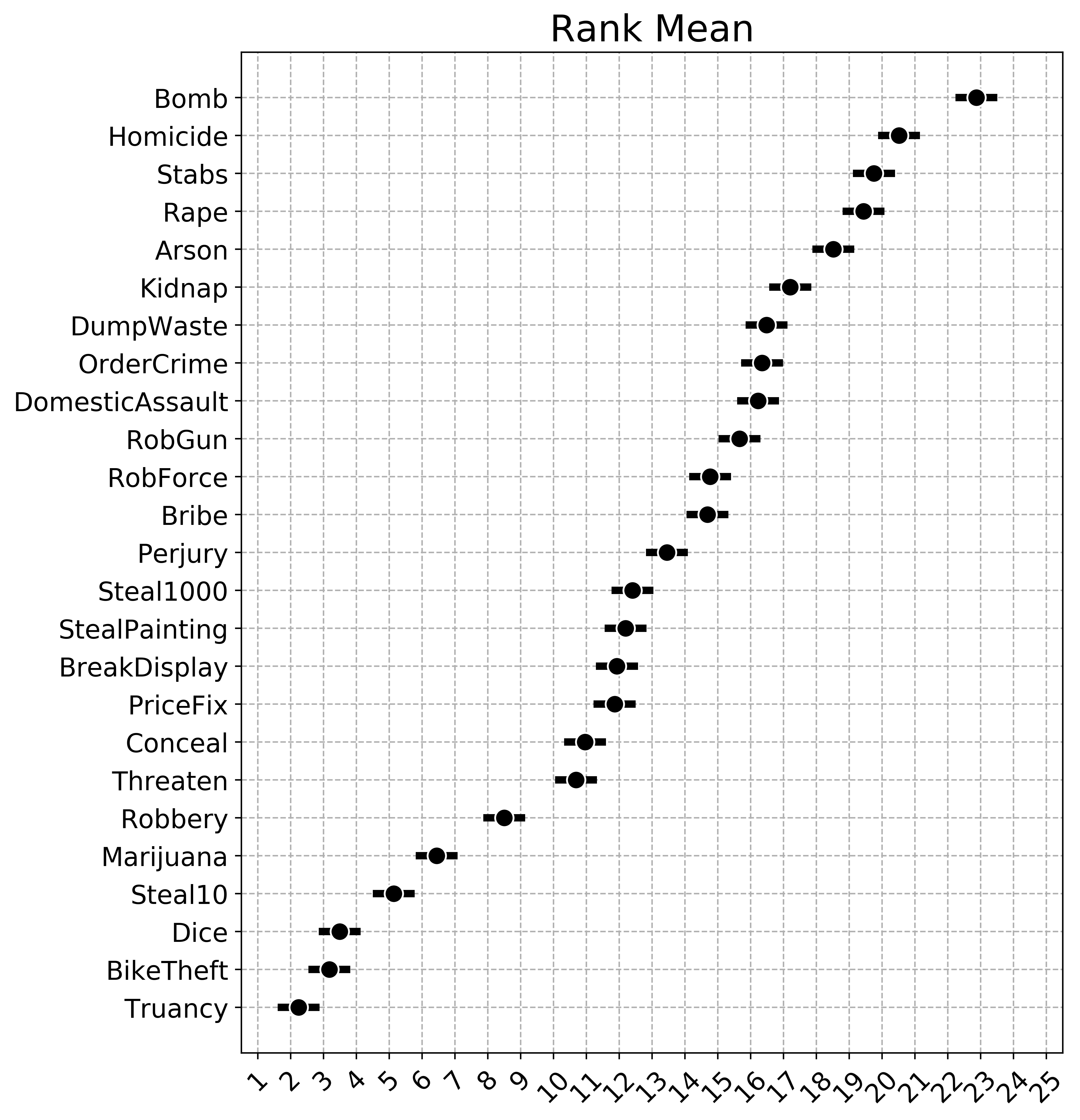
I have created some python code to follow along and apply these same customer lifetime value estimates to chronic offender data. Most examples of weighting crime harm apply it to spatial areas (Mitchell, 2019; Wheeler & Reuter, 2021), but you can apply it the same to chronic offender lists (Liggins et al., 2019).

Example Criminal Lifetime Value in Python

First, install the lifetimes python library – Cam’s documentation is excellent and makes the data manipulation/modelling quite simple.

Here I load in the transaction level crime data, e.g. it just have person A, 1/5/1960, 1000, where the 1000 is a crime seriousness index created by Wolfgang. Then the lifetimes package has some simple functions to turn our data into the frequency/recency format.

Note that for these models, you drop the first event in the series. To build a model to do train/test, I also split the data into evens before 1962, and use 1962 as the holdout test period.

import lifetimes as lt
import pandas as pd

# Just the columns from dataset II
# ID, SeriousScore, Date
df = pd.read_csv('PhilData.csv')
df['Date'] = pd.to_datetime(df['Date'])

# Creating the cumulative data
# Having holdout for one year in future
sd = lt.utils.calibration_and_holdout_data(df,'ID','Date',
              calibration_period_end='12-31-1961',
              observation_period_end='12-31-1962',
              freq='M',
              monetary_value_col='SeriousScore')

# Only keeping people with 2+ events in prior period
sd = sd[sd['frequency_cal'] > 0].copy()
sd.head()

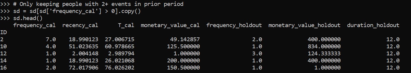
Recency_cal is how many months since a prior crime (starting in 1/1/1962), frequency is the total number of events (minus 1, so number of repeat events technically), and the monetary_value_cal here is the average of the crime seriousness across all the events. The way this function works, the variables with the subscript _cal are in the training period, and _holdout are events in the 1962 period. For subsequent models I subset out people with at least 2 events total in the modeling.

Now we can fit a model to estimate the predicted number of future crimes a person will commit – so this does not take into account the seriousness of those crimes. The final groupby statement shows the predicted number of crimes vs those actually committed, broken down by number of crimes in the training time period. You can see the model is quite well calibrated over the entire sample.

# fit BG model
bgf = lt.BetaGeoFitter(penalizer_coef=0)
bgf.fit(sd['frequency_cal'],sd['recency_cal'],sd['T_cal'])

# look at fit of BG model
t = 12
sd['pred_events'] = bgf.conditional_expected_number_of_purchases_up_to_time(t, sd['frequency_cal'], sd['recency_cal'],sd['T_cal'])
sd.groupby('frequency_cal',as_index=False)[['frequency_holdout','pred_events']].sum() # reasonable

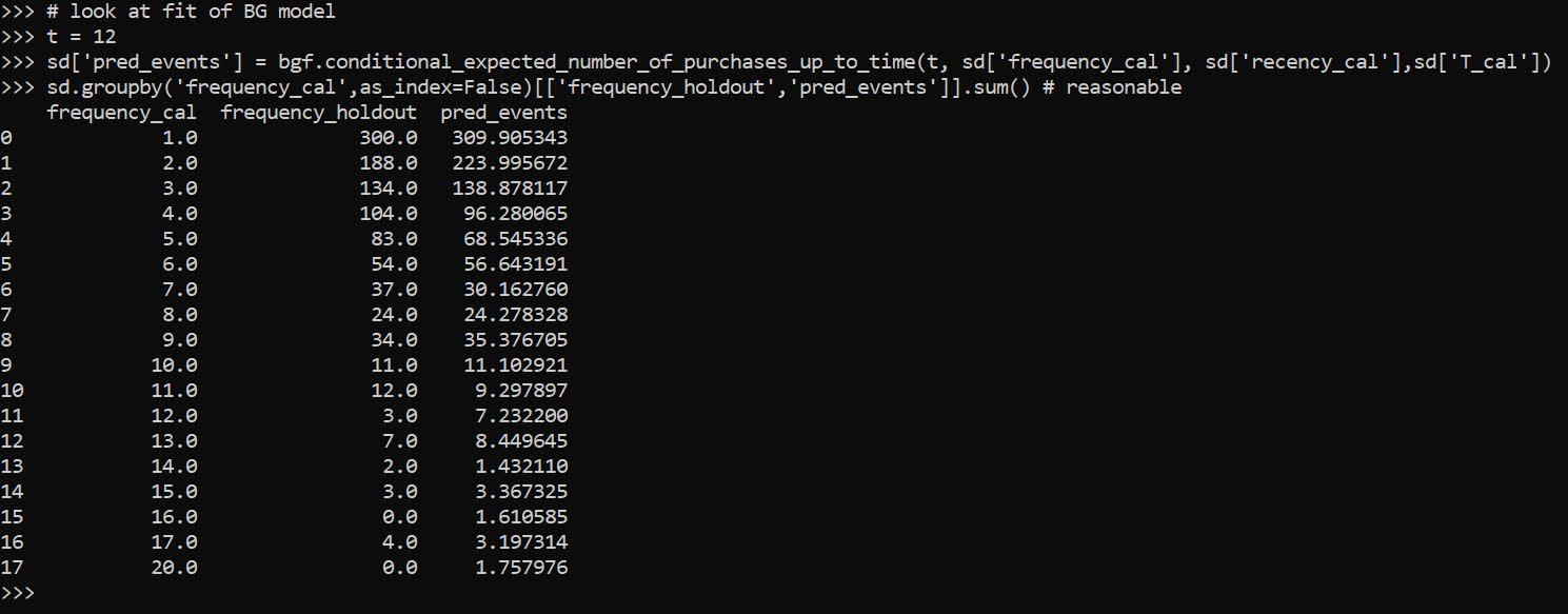
Now we can fit a model to estimate the average crime severity score for an individual as well. Then you can project a future cumulative score for an offender (here over a horizon of 1 year), by multiple the predicted number of events times the estimate of the average severity of the events, what I label as pv here:

# See conditional seriousness
sd['pred_ser'] = ggf.conditional_expected_average_profit(
                              sd['frequency_cal'],
                              sd['monetary_value_cal'])

sd['pv'] = sd['pred_ser']*sd['pred_events']
sd['cal_tot_val'] = sd['monetary_value_holdout']*sd['frequency_holdout']
# Not great correlation, around 0.2
vc = ['frequency_holdout','monetary_value_holdout','cal_tot_val','pred_events','pv']
sd[vc].corr()

The correlation between pv and the holdout cumulative crime severity cal_tot_val, is not great at 0.26. But lets look at this relative to the more typical approach analysts will do, simply rank prior offenders based on either total number of events or the crime seriousness:

# Lets look at this method via just ranking prior
# seriousness or frequency
sd['rank_freq'] = sd['frequency_cal'].rank(method='first',ascending=True)
sd['rank_seri'] = (sd['monetary_value_cal']*sd['frequency_cal']).rank(method='first',ascending=True)
vc += ['rank_freq','rank_seri']
sd[vc].corr()[vc[-3:]]

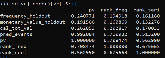
So we can see that pv outperforms ranking based on total crimes (rank_freq), or ranking based on the cumulative serious score for offenders (rank_seri) in terms of the correlation for either the total number of future events or the cumulative crime harm.

If we look at capture rates, e.g. pretend we highlight the top 50 chronic offenders for intervention, we can see the criminal lifetime value pv estimate outperforms either simple ranking scheme by quite a bit:

# Look at capture rates by ranking
topn = 50
res_summ = []
for v in vc[-3:]:
    rank = sd[v].rank(method='first',ascending=False)
    locv = sd[rank <= topn].copy()
    tot_crimes = locv['frequency_holdout'].sum()
    tot_ser = locv['cal_tot_val'].sum()
    res_summ.append( [v,tot_crimes,tot_ser,topn] )

res_df = pd.DataFrame(res_summ,columns=['Var','TotCrimes','TotSer','TotN'])
res_df

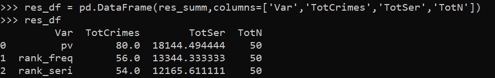
In terms of the seriousness projection, it is reasonably well calibrated over the entire sample, but has a very tiny variance – it basically just predicts the average crime serious score over the sample and assigns that as the prediction going forward:

# Cumulative stats over sample reasonable
# variance much too small
sd[['cal_tot_val','pv']].describe()

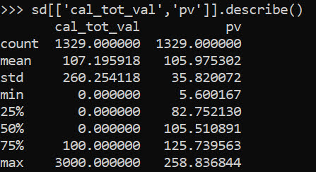
So what this means is that if say Chicago READI wanted to do estimates to reasonably justify the max dollar cost for their program (over a large number of individuals) that would be reasonable. And this is how most marketing people use this info, average benefits of retaining a customer.

For individual projections though, e.g. I think OffenderB will generate between [low,high] crime harm in the next year, this is not quite up to par. I am hoping though to pursue these models further, maybe either in a machine learning/regression framework to estimate the parameters directly, or to use mixture models in an equivalent way that marketers use “segmentation” to identify different types of customers. Knowing the different way people have formulated models though is very helpful to be able to build a machine learning framework, which you can incorporate covariates.

References

Amending the WDD test to incorporate Harm Weights

So I received a question the other day about amending my and Jerry Ratcliffe’s Weighted Displacement Difference (WDD) test to incorporate crime harms (Wheeler & Ratcliffe, 2018). This is a great idea, but unfortunately it takes a small bit of extra work compared to the original (from the analysts perspective). I cannot make it as simple as just piping in the pre-post crime weights into that previous spreadsheet I shared. The reason is a reduction of 10 crimes with a weight of 10 has a different variance than a reduction of 25 crimes with a weight of 4, even though both have the same total crime harm reduction (10*10 = 4*25).

I will walk through some simple spreadsheet calculations though (in Excel) so you can roll this on your own. HERE IS THE SPREADSHEET TO DOWNLOAD TO FOLLOW ALONG. What you need to do is to calculate the traditional WDD for each individual crime type in your sample, and then combine all those weighted WDD’s estimates in the end to figure out your crime harm weighted estimate in the end (with confidence intervals around that estimated effect).

Here is an example I take from data from Worrall & Wheeler (2019) (I use this in my undergrad crime analysis class, Lab 6). This is just data from one of the PFA areas and a control TAAG area I chose by hand.

So first, go through the motions for your individual crimes in calculating the point estimate for the WDD, and then also see the standard error of that estimate. Here is an example of piping in the data for thefts of motor vehicles. The WDD is simple, just pre-post crime counts. Since I don’t have a displacement area in this example, I set those cells to 0. Note that the way I calculate this, a negative number is a good thing, it means crime went down relative to the control areas.

Then you want to place those point estimates and standard errors in a new table, and in those same rows assign your arbitrary weight. Here I use weights taken from Ratcliffe (2015), but these weights can be anything. See examples in Wheeler & Reuter (2020) for using police cost of crime estimates, and Wolfgang et al. (2006) for using surveys on public perceptions of severity. Many of the different indices though use sentencing data to derive the weights. (You could even use negative weights and the calculations here all work, say you had some positive data on community interactions.)

Now we have all we need to calculate the harm-weighted WDD test. The big thing here to note is that the variance of Var(x*harm_weight) = Var(x)*harm_weight^2. So that allows me to use all the same machinery as the original WDD paper to combine all the weights in the end. So now you just need to add a few additional columns to your spreadsheet. The point estimate for the harm reduction is simply the weight multiplied by the point estimate for the crime reduction. The variance though you need to square the standard error, and square the weight, and then multiply those squared results together.

Once that is done, you can pool the harm weighted stats together, see the calculations below the table. Then you can use all the same normal distribution stuff from your intro stats class to calculate z-scores, p-values, and confidence intervals. Here are what the results look like for this particular example.

I think this is actually a really good idea to pool results together. Many place based police interventions are general, in that you might expect them to reduce multiple crime types. Various harm scores are a good way to pool the results, instead of doing many individual tests. A few caveats though, I have not done simulations like I did in the WDD peer reviewed paper, I believe these normal approximations will do OK under the same circumstances though that we suggest it is reasonable to do the WDD test. You should not do the WDD test if you only have a handful of crimes in each area (under 5 in any cell in that original table is a good signal it is too few of crimes).

These crime count recommendations I think are likely to work as well for weighted crime harm. So even if you give murder a really high weight, if you have fewer than 5 murders in any of those original cells, I do not think you should incorporate it into the analysis. The large harm weight and the small numbers do not cancel each other out! (They just make the normal approximation I use likely not very good.) In that case I would say only incorporate individual crimes that you are OK with doing the WDD analysis to begin with on their own, and then pool those results together.

Sometime I need to grab the results of the hot spots meta-analysis by Braga and company and redo the analysis using this WDD estimate. I think the recent paper by Braga and Weisburd (2020) is right, that modeling the IRR directly makes more sense (I use the IRR to do cost-benefit analysis estimates, not Cohen’s D). But even that is one step removed, so say you have two incident-rate-ratios (IRRs), 0.8 and 0.5, the latter is bigger right? Well, if the 0.8 study had a baseline of 100 crimes, that means the reduction is 100 - 0.8*100 = 20, but if the 0.5 study had a baseline of 30 crimes, that would mean a reduction of 30 - 0.5*30 = 15, so in terms of total crimes is a smaller effect. The WDD test intentionally focuses on crime counts, so is an estimate of the actual number of crimes reduced. Then you can weight those actual crime decreases how you want to. I think worrying about the IRR could even be one step too far removed.

References

Conjoint Analysis of Crime Rankings

So part of my recent research mapping crime harm spots uses cost of crime estimates relevant to police departments (Wheeler & Reuter, 2020). But a limitation of this is that cost of crime estimates are always somewhat arbitrary.

For a simple example, those cost estimates are based mostly on people time by the PD to respond to crimes and devote investigative resources. Many big city PDs entirely triage crimes like breaking into vehicles though. So based on PD response the cost of those crimes are basically $0 (especially if PDs have an online reporting system).

But I don’t think the public would agree with that sentiment! So in an act of cognitive dissonance with my prior post, I think asking the public is likely necessary for police to be able to ultimately serve the publics interest when doing valuations. For some ethical trade-offs (like targeting hot spots vs increasing disproportionate minority contact, Wheeler, 2019) I am not sure there is any other reasonable approach than simply getting a bunch of peoples opinions.

But that being said, I suspected that these different metrics would provide pretty similar rankings for crime severity overall. So while it is criminology 101 that official crime and normative perceptions of deviance are not a perfect 1 to 1 mapping, most folks (across time and space) have largely similar agreement on the severity of different crimes, e.g. that assault is worse than theft.

So what I did was grab some survey ranking of crime data from the original source of crime ranking that I know of, Marvin Wolfgang’s supplement to the national crime victimization survey (Wolfgang et al., 2006). I have placed all the code in this github folder to replicate. And in particular check out this Jupyter notebook with the main analysis.

Conjoint Analysis of Crime Ranks

This analysis is often referred to as conjoint analysis. There are a bunch of different ways to conduct conjoint analysis – some ask folks to create a ranked list of items, others ask folks to choose between a list of a few items, and others ask folks to rank problems on a Likert item 1-5 scale. I would maybe guess Likert items are the most common in our field, see for example Spelman (2004) using surveys of asking people about disorder problems (and that data is available to, Taylor, 2008).

The Wolfgang survey I use here is crazy complicated, see the codebook, but in a nutshell they had an anchoring question where they assigned stealing a bike to a value of 10, and then asked folks to give a numeric score relative to that theft for a series of 24 other crime questions. Here I only analyze one version of the questionnaire, and after eliminating missing data there are still over 4,000 responses (in 1977!).

So you could do analyze those metric scores directly, but I am doing the lazy route and just doing a rank ordering (where ties are the average rank) within person. Then conjoint analysis is simply a regression predicting the rank. See the notebook for a more detailed walkthrough, so this just produces the same analysis as looking at the means of the ranks.

About the only thing I do different here than typical conjoint analysis is that I rescale the frequency weights (just changes the degrees of freedom for standard error estimates) to account for the repeated nature of the observations (e.g. I treat it like a sample of 4000 some observations, not 4000*25 observations). (I don’t worry about the survey weights here.)

To test my assertion of whether these different ranking systems will be largely in agreement, I take Jerry’s crime harm paper (Ratcliffe, 2015), which is based on sentencing guidelines, and map them as best I could to the Wolfgang questions (you could argue with me some though on those assements – and some questions don’t have any analog, like a company dumping waste). I rescaled the Wolfgang rankings to be in a range of 1-14, same as Jerry’s, instead of 1-25.

Doing a more deep dive into the Wolfgang questions, there are definately different levels in the nature of the questions you can tease out. Folks clearly take into account both harm to the victim and total damages/theft amounts. But overall the two systems are fairly correlated. So if an analyst wants to make crime harm spots now, I think it is reasonable to use one of these ranking systems, and then worry about getting the public perspective later on down the line.

The Wolfgang survey is really incredible. In this regression framework you can either adjust for other characteristics (e.g. it asks about all the usual demographics) or look at interactions (do folks who were recently victimized up their scores). So this is really just scratching the surface. I imagine if someone redid it with current data many of the metrics would be similar as well, although if I needed to do this I don’t think I would devise something as complicated as this, and would ask people to rank a smaller set of items directly.

References

  • Ratcliffe, J.H. (2015). Towards an index for harm-focused policing. Policing: A Journal of Policy and Practice, 9(2), 164-182.
  • Spelman, W. (2004). Optimal targeting of incivility-reduction strategies. Journal of Quantitative Criminology, 20(1), 63-88.
  • Taylor, R.B. (2008). Impacts of Specific Incivilities on Responses to Crime and Local Commitment, 1979-1994: [Atlanta, Baltimore, Chicago, Minneapolis-St. Paul, and Seattle]. https://doi.org/10.3886/ICPSR02520.v1
  • Wheeler, A.P., & Reuter, S. (2020). Redrawing hot spots of crime in Dallas, Texas. https://doi.org/10.31235/osf.io/nmq8r
  • Wheeler, A.P. (2019). Allocating police resources while limiting racial inequality. Justice Quarterly, Online First.
  • Wolfgang, M.E., Figlio, R.M., Tracy, P.E., and Singer, S.I. (2006). National Crime Surveys: Index of Crime Severity, 1977. https://doi.org/10.3886/ICPSR08295.v1