Some theory behind the likability of XKCD style charts


Recently on the stackexchange sites there was a wave of questions regarding how to make XKCD style charts (see example above). Specifically, the hand-drawn imprecise look about the charts.

There also appear to be a variety of other language examples floating around, like MATLAB, D3 and Python.

What is interesting about these exchanges, in some highly scientific/computing communities, is that they are excepted (that was a weird Freudian slip) accepted with open arms. Some dogmatic allegiance to Tufte may consider these to be at best chart junkie, and at worst blatant distortions of data (albeit minor ones). For an example of the fact that at least the R community on stackoverflow is aware of such things, see some of the vitriol to this question about replicating some aesthetic preferences of gradient backgrounds and rounded edges (available in Excel) in R. So what makes these XKCD charts different? Certainly the content of the information in XKCD comics is an improvement over typical horrific 3d pie charts in Excel, but this doesn’t justify there use.

Wood et al. (2012) provide some commentary as to perhaps why people like the charts. Such hypothesis include that the sketchy rendering evokes some mental model of simplicity, and thus reduces barriers to first interpreting the image. The actual sketchy rendering also makes one focus on more obvious global characteristics of the graphic, and thus avoid spending attention on minor imperceivable details. This should also lead into why it is a potentially nice tool to visualize uncertainty in the data presented. The concept of simplifying and generalizing geographic shapes has been known for awhile in cartography (I’m skeptical it is much known in the more general data-viz community), but this is a bit of a unique extension.

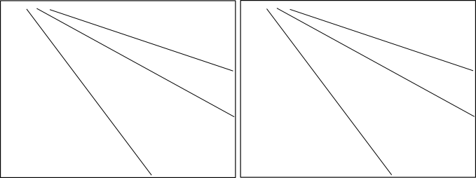
Besides the implementations noted at the prior places, they also provide a library, Handy for making sketchy drawings from any graphics produced in Processing. Below are two examples.


So there isn’t just a pretty picture behind the logic of why everyone likes the XKCD style charts. It is a great example of the divide between classical statistical graphics (ala Tufte and Cleveland) versus current individuals within journalism and data-viz who attempt to make charts aesthetically pleasing, attention grabbing, and for the masses. Wood and company take great lengths to show the relative error in the paper cited when using such sketchy rendering, but weighing the benefits of readability vs. error in graphics is a difficult question to address going forward.


Citations

The leaning tower optical illusion: Is it applicable to statistical graphics?


Save in the memory banks whether the slope of the lines in the left hand panel appear similar, smaller or larger than the slope of the lines in the right hand panel.

I enjoy reading about optical illusions, both purely because I think they are neat and there applicability to how we present and perceive information in statistical graphics. A few examples I am familiar with are;

  • The Rubin Vase optical illusion in which it is difficult to distinguish between what object is the background and which is the foreground. This is applicable to making clear background/foreground seperation between grid lines and chart elements.
  • Change blindness, which makes it difficult to interpret animated graphics that do not have smooth, continous transitions between chart states.
  • Mach bands, where the color of an object is perceived differently given the context of the surrounding colors. I recently came across one of the most dramatic examples of this at the very cool mighty optical illusion site. I actually went and edited the image in that example to make sure there was no funny business it was so dramatic an effect! Image included below.


I was recently pointed to a new (to me) example of an optical illusion, the leaning tower illusion, in a paper by Kingdom, Yoonessi & Gheorghiu (2007) (referred via the Freakonometrics blog).


Although I suggest to read the article (it is very brief) – to sum it up both pictures above are identical, although the tower on the right appears to be leaning more to the right. Although the pictures are seperate (and have some visual distinction) our minds interpret them in the same “plane”. And hence objects that are further away in the distance should not be parallel but should actually converge within the image.

Off-the-cuff this reminded me of the Ponzo illusion, where our minds know that the lines are still running parallel, and our perception of other surrounding elements changes conditional on that dominant parallel lines pattern. Here is another good example of this from the mighty optical illusions site (actually I did not know the name of this effect – and when I googled subway tile illusion this is the site that came up – and I’m glad I found it!)

Is this applicable to statistical graphics though? One of the later images in the Perception article appear to be potentially more reminiscent of a small multiple line chart (and we all know I strongly advocate for the use of small multiple charts).


We do know that interpreting the distance between sloping lines is difficult (as elaborated on in some of Cleveland’s work), but this is different in that potentially our perception of the parallelness of lines between panels in a small multiple is distorted based the directions of lines within the panel. Off-hand though we may expect that the context doesn’t exactly carry-over, there is no visual schematic in 2d statistical graphics that lines are running further from our perspective. So to test this out I attempted to create some settings in small multiple line panels that might cause similar optical illusions.

So, going back to the picture at the beginning of the article, here are those same lines superimposed on the original picture. My personal objectivity to tell if these result in visual distortions is gone at this point, but at best I could only conjure up perhaps some slight distortion between panels (which is perhaps no worse than our ability to effectively perceive slopes accurately anyway).

I think along these lines one could come up with some more examples where between panel comparisons for line graphs in small multiples produce such distortions, but I was unable to produce anything compelling in some brief tries (so let me know if you come across any examples where such distortions occur!) Simply food for thought though at this point.

I do think though that the Ponzo scheme can be illustrated with essentially the same graphic.


It isn’t as dramatic as the subway tile example, but I do think it appears the positive sloping line where the negative sloping lines converge at the top of the image appears larger than the line in space and the bottom right of the image.

I suspect this could actually occur in real life graphics in which we have error bars superimposed on a graph with several lines of point estimates. If the point estimates start at a wide interval and then converge, it may produce a similar illusion that the error bars appear larger around the point estimates that are closer together. Again though I produced nothing real compelling in my short experimentation.

Example (good and bad) uses of 3d choropleth maps

A frequent critique of choropleth maps is that, in the process of choosing color bins, one can hide substantial variation within each of the bins . An example of this is in this critique of a map in the Bad maps thread on the GIS stackexchange site.  In particular, Laurent argues that the classification scheme (in that example map) is misleading because China’s population (1.3 billion) and Indonesia’s population (0.2 billion) are within the same color bin although they have noteworthy differences in their population.

I think it is a reasonable note, and such a difference would be noteworthy in a number of contexts. One possible solution to this problem is by utilizing 3d choropleth maps, where the height of the bar maps to a quantitative value.  An example use of this can be found at Alasdair Rae’s blog, Daytime Population in the United States.

The use of 3d allows one to see the dramatic difference in daytime population estimates between the cities (mainly on the east coast).  Whereas a 2d map relying on a legend can’t really demonstrate the dramatic magnitude of differences between legend items like that.

I’m not saying a 3d map like this is always the best way to go. Frequent critiques are that the bars will hide/obstruct data. Also it is very difficult to really evaluate where the bars lie on the height dimension. For an example of what I am talking about, see the screen shot used for this demonstration,  A Historical Snapshot of US Birth Trends, from ge.com (taken from the infosthetics blog).

If you took the colors away, would you be able to tell that Virginia is below average?

Still, I think used sparingly and to demonstrate dramatic differences they can be used effectively.  I give a few more examples and/or reading to those interested below.

References

Ratti, Carlo, Stanislav Sobolevsky, Francesco Calabrese, Clio Andris, Jonathan Reades, Mauro Martino, Rob Claxton & Steven H. Strogatz. (2010) Redrawing the map of Great Britain from a Network of Human Interactions. PLoS ONE 5(12). Article is open access from link.

This paper is an example of using 3d arcs for visualization.

Stewart, James & Patrick J. Kennelly. 2010. Illuminated choropleth maps. Annals of the Association of American Geographers 100(3): 513-534.

Here is a public PDF by one of the same authors demonstrating  the concept. This paper gives an example of using 3d choropleth maps, and in particular is a useful way to utilize a 3d shadow effect that slightly enhances distinguishing differences between two adjacent polygons. This doesn’t technique doesn’t really map height to a continuous variable though, just uses shading to distinguish between adjacent polygons.

Other links of interest

GIS Stackexchange question – When is a 3D Visualisation in GIS Useful?

A cool example of utilizing 3d in kml maps on the GIS site by dobrou, Best practices for visualizing speed.

Alasdair Rae’s blog has several examples of 3d maps besides the one I linked to here, and I believe he was somehow involved in making the maps associated with this Centre for Cities short clip (that includes 3d maps).

If you have any other examples where you thought the use of 3d maps (or other visualizations) was useful/compelling let me know in the comments.

Edit: I see looking at some of my search traffic that this blog post is pretty high up for “3d choropleth” on a google image search already. I suspect that may mean I am using some not-well adopted terminology, although I don’t know what else to call these types of maps.

The thematic mapping blog calls them prism maps (and is another place for good examples). Also see the comment by Jon Peltier for that post, and the subsequent linked blog post by the guys at Axis maps (whose work I really respect), Virtual Globes are a seriously bad idea for thematic mapping.

Edit2: I came across another example, very similar to Alasdair Rae’s map produced by the New York Times, Where America Lives. Below is a screen shot (at the link they have an interactive map). Referred to by the folks at OCSI, and they call this type of map a “Spike Map”.