When viewing past synthetic control results, one of things that has struck me is that the matching of the pre-trends is really good — almost too good in many cases (appears to be fitting to noise, although you may argue that is a feature in terms of matching exogenous shocks). For example, if you end up having a pre-treatment series of 10 years, and you have a potential donor pool the size of 30, you could technically pick 10 of them at random, fit a linear regression predicting the 10 observations in the treated unit, based on 10 covariates of the donor pool outcomes over the same pre time period, and get perfect predictions (ignoring the typical constraints one places on the coefficients).

So how do we solve that problem? One solution is to use regularized regression results (e.g. ridge regression, lasso), when the number of predictors is greater than the number of observations. So I can cast the matching procedure into a regression problem to generate the weights. Those regression procedures are typically used for forecasting, but don’t have well defined standard errors, and so subsequently are typically only used for point forecasts. One way to make inferences though is to generate the synthetic weights (here using lasso regression), and then use conformal prediction intervals to do our hypothesis testing of counterfactual trends.

Here I walk through an example using state panel crime data in R, full code and data can be downloaded here.

A Synthetic Control Example

So first, these are the packages we need to replicate the results. conformalInference is not on CRAN yet, so use devtools to install it.

#library(devtools)
#install_github(repo="ryantibs/conformal", subdir="conformalInference")
library(conformalInference)
library(glmnet)
library(Synth)

Then I have prepped a nice state panel dataset of crime rates and counts from 1960 through 2014. I set a hypothetical treatment start year in 2005 just so I have a nice 10 years post data for illustration. That is a pretty good length pre-panel though, and a good number of potential donors.

MyDir <- "C:\\Users\\axw161530\\Desktop\\SynthIdeas"
setwd(MyDir)

TreatYear <- 2005

LongData <- read.csv("CrimeStatebyState_Edited.csv")
summary(LongData)

Next I prep my data, currently it is in long panel format, but I need it in wide format to fit the regression equations I want. I am just matching on violent crime rates here. I take out NY, as it is missing a few years of data. (This dataset also includes DC.) Then I split it up into my pre intervention and post intervention set.

#Changing the data to wide for just the violent offenses
wide <- LongData[,c('State','Year','Violent.Crime.rate')]
names(wide)[3] <- 'VCR'
wide <- reshape(wide, idvar="Year", timevar="State", direction="wide")
summary(wide)
#Take out NY because of NAs
wide <- wide[,c(1:33,35:52)]

wide_pre <- as.matrix(wide[wide$Year < TreatYear,])
wide_post <- as.matrix(wide[wide$Year >= TreatYear,])

Now onto the good stuff, we can estimate our lasso regression using the pre-data to get our weights. This constrains the coefficients to be positive and below 1. But does not have the constraint they sum to 1. I just choose Alabama as an example treated unit — I intentionally chose a state and year that should not have any effects for illustration and to check the coverage of my technique vs more traditional analyses.

You can see in my notes this is different than traditional synth in that it has an intercept as well. I was surprised, but the predictions in sample were really bad without the intercept no matter how I sliced it.

res <- glmnet(x=wide_pre[,3:51],y=wide_pre[,2],family="gaussian",
       lower.limits=0,upper.limits=1,intercept=TRUE,standardize=FALSE,
       alpha=1) #need the intercept, predictions suck otherwise

Even though this does not constrain the coefficients to sum to 1, it ends up with weights really close to that ideal anyway (sum of the non-intercept coefficients is just over 1.01). When I use crossvalidation it does not choose weights that sum to unity, but in sample the above code and the cv.glmnet are really similar in terms of predictions.

co_ridge <- as.matrix(coef(res))
fin <- co_ridge[,"s99"]
active <- fin[fin > 0] #Does not include intercept

If you print active we then have for our state weights (and the intercept is pretty tiny, -22). So not quite sure why eliminating the intercept was causing such problems in this example. So North Carolina just sneaks in, but otherwise the synthetic control is a mix of Arkansas, California, Kentucky, and Texas. The intercept is just a level shift, so we are still matching curves otherwise, so that does not bother me very much.

VCR.AR 0.2078156362
VCR.CA 0.1201658279
VCR.IL 0.1543015666
VCR.KY 0.2483613907
VCR.NC 0.0002896238
VCR.TX 0.2818272850

If we look at our predictions for the pre-time period, Alabama had the typical crime path, with a big raise going into the early 90’s and then a fall afterward (black line), and our in-sample predictions from the lasso regression are decent.

pre_pred <- predict(res,newx=wide_pre[,3:51],s=min(res$lambda)) #for not cv results

plot(wide_pre[,1],wide_pre[,2],type='l',xlab='',ylab='Violent Crime Rate per 100,000')
points(wide_pre[,1],pre_pred,bg='red',pch=21) #Not too shabby
legend(1960,800,legend=c("Observed Albama","Predicted"),col=c("black","black"), pt.bg=c("black","red"), lty=c(1,NA), pch=c(NA,21))

Now to evaluate post intervention, we are going to generate conformal prediction intervals using a jackknife approach. Basically doing all the jazz of above, but leaving one pre year out at a time, and trying to predict Alabama’s violent crime rate for that left out year. Repeat that same process for all prior years, and we can get a calculation of the standard error of our prediction. Then apply that standard error to future years, so we can tell if the observed trend is different than the counterfactual we estimated (given the counterfactual has errors). I generate both 90% prediction intervals, as well as 99% prediction intervals.

train_fun <- function(x, y, out=NULL){
  return( glmnet(x,y,alpha=1,standardize=FALSE,intercept=TRUE,nlambda=100,
                lower.limits=0,upper.limits=1,family="gaussian")
  )
}

pred_fun = function(out, newx) {
    return(predict(out, newx, s=min(out$lambda)))
}

limits_10 <- conformal.pred.jack(x=wide_pre[,3:51],y=wide_pre[,2],x0=wide_post[,3:51],
                                 train.fun=train_fun,predict.fun=pred_fun,alpha=0.10,
                                 verbose=TRUE)

limits_01 <- conformal.pred.jack(x=wide_pre[,3:51],y=wide_pre[,2],x0=wide_post[,3:51],
               train.fun=train_fun,predict.fun=pred_fun,alpha=0.01,
               verbose=TRUE)

plot(wide_post[,1],wide_post[,2],type='l',ylim=c(150,650),xlab='',ylab='Violent Crime Rate per 100,000')
points(wide_post[,1],post_pred,bg='red',pch=21)
lines(wide_post[,1],limits_10$lo,col='grey')
lines(wide_post[,1],limits_10$up,col='grey')
lines(wide_post[,1],limits_01$lo,col='grey',lwd=3)
lines(wide_post[,1],limits_01$up,col='grey',lwd=3)
legend("topright",legend=c("Observed Albama","Predicted","90% Pred. Int.","99% Pred. Int."),cex=0.7,
       col=c("black","black","grey","grey"), pt.bg="red", lty=c(1,NA,1,1), pch=c(NA,21,NA,NA), lwd=c(1,1,1,3))

Then at the end of the above code snippet I made a plot. Black line is observed for Alabama from 05-14. Red dots are the estimated counterfactual based on the pre-weights. The lighter grey lines are then the prediction intervals. So we can see it is just outside the 90% intervals 3 times in the later years (would only expect 1 time), but all easily within the 99% intervals.

Note these are prediction intervals, not confidence intervals. Thinking about it I honestly don’t know whether we want prediction or confidence intervals in this circumstance, but prediction will be wider.

So this approach just matches on the pre-treated same outcome observations. To match on additional covariates, you can add them in as rows into the pre-treatment dataset (although you would want to normalize the values to a similar mean and standard deviation as the pre-treated outcome series).

You may also add in other covariates, like functions of time (although this changes the nature of the identification). So for example say you incorporate a linear and quadratic trend in time, and lasso only chooses those two time factors and no control areas. You are doing something more akin to interrupted time series analysis at that point (the counterfactual is simply based on your estimate of the pre-trend). Which I think is OK sometimes, but is quite different than using control areas to hopefully capture random shocks.

Comparing to Traditional Synth results

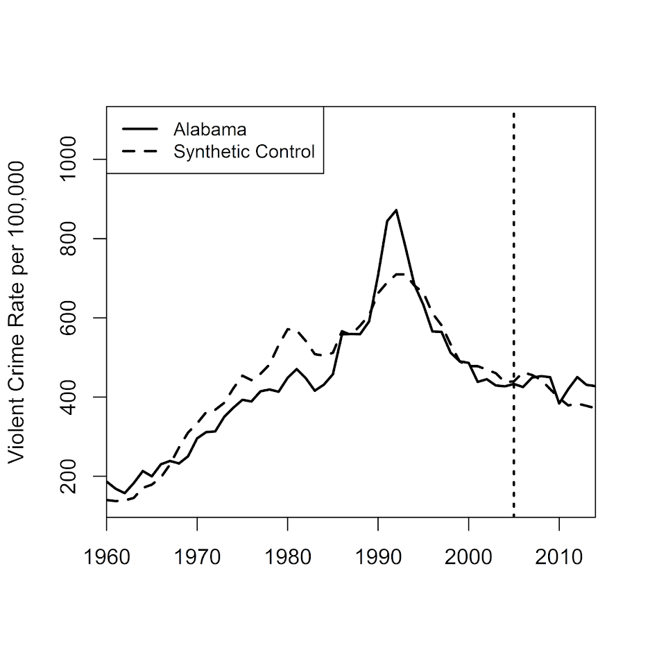
To see whether my error intervals are similar to the placebo approach, I used the old school synth R package. It isn’t 100% comparable, as it makes you match on at least one covariate, so here I choose to also match on the average logged population over the pre-treatment period.

#NY is missing years
LongData_MinNY <- LongData[as.character(LongData$State) != "NY",c("State","Year","Violent.Crime.rate","Population")]
LongData_MinNY$StateNum <- as.numeric(LongData_MinNY$State)
LongData_MinNY$State <- as.character(LongData_MinNY$State)
LongData_MinNY$LogPop <- log(LongData_MinNY$Population)    

state_nums <- unique(LongData_MinNY$StateNum)
    
dataprep.out <- dataprep(foo = LongData_MinNY,
                         dependent = "Violent.Crime.rate",
                         predictors = c("LogPop"),
                         unit.variable = "StateNum",
                         unit.names.variable = "State",
                         time.variable = "Year",
                         treatment.identifier = 2,
                         controls.identifier = state_nums[!state_nums %in% 2],
                         time.optimize.ssr = 1960:(TreatYear-1),
                         time.predictors.prior = 1960:(TreatYear-1),
                         time.plot = 1960:2014
                         )

synth_res <- synth(dataprep.out)
synth_tables <- synth.tab(dataprep.res = dataprep.out, synth.res = synth_res)
synth_tables$tab.w #a bunch of little weights across the board
path.plot(synth.res = synth_res, dataprep.res = dataprep.out, tr.intake=TreatYear,Xlab='',Ylab='Violent Crime Rate per 100,000',
      Legend=c("Alabama","Synthetic Control"), Legend.position=c("topleft"))

Looking at the weights, it is a bunch of little ones for many different states. Looking at the plot, it doesn’t appear to be any better fit than the lasso approach.

And then I just do the typical approach and use placebo checks to do inference. I loop over my 49 placebos (-1 state for NY, but +1 state because this list includes DC).

#Dataframes to stuff the placebos check results into
Predicted <- data.frame(dataprep.out$Y0plot %*% synth_res$solution.w)
names(Predicted) <- "TreatPred"

Pred_MinTreat <- data.frame(TreatPred = Predicted$TreatPred - LongData_MinNY[LongData_MinNY$StateNum == 2,"Violent.Crime.rate"])

#Now I just need to loop over the other states and collect their results for the placebo tests

placebos <- state_nums[!state_nums %in% 2]
for (i in placebos){
  dataprep.plac <- dataprep(foo = LongData_MinNY,
                           dependent = "Violent.Crime.rate",
                           predictors = c("LogPop"),
                           unit.variable = "StateNum",
                           unit.names.variable = "State",
                           time.variable = "Year",
                           treatment.identifier = i,
                           controls.identifier = state_nums[!state_nums %in% i],
                           time.optimize.ssr = 1960:(TreatYear-1),
                           time.predictors.prior = 1960:(TreatYear-1),
                           time.plot = 1960:2014
  )
  synth_resP <- synth(dataprep.plac)
  synth_tablesP <- synth.tab(dataprep.res = dataprep.plac, synth.res = synth_resP)
  nm <- paste0("S.",i)
  Predicted[,nm] <- dataprep.plac$Y0plot %*% synth_resP$solution.w
  Pred_MinTreat[,nm] <- Predicted[,nm] - LongData_MinNY[LongData_MinNY$StateNum == i,"Violent.Crime.rate"]
}

If you look at the synth estimates for Alabama (grey circles), they are almost exactly the same as the lasso predictions (red circles), even though the weights are very different.

PredRecent <- Predicted[1960:2014 >= TreatYear,]
DiffRecent <- Pred_MinTreat[1960:2014 >= TreatYear,]

plot(wide_post[,1],wide_post[,2],type='l',ylim=c(100,700),xlab='',ylab='Violent Crime Rate per 100,000')
points(wide_post[,1],post_pred,bg='red',pch=21)
lines(wide_post[,1],limits_10$lo,col='grey')
lines(wide_post[,1],limits_10$up,col='grey')
lines(wide_post[,1],limits_01$lo,col='grey',lwd=3)
lines(wide_post[,1],limits_01$up,col='grey',lwd=3)
points(wide_post[,1],PredRecent$TreatPred,bg='grey',pch=21)
legend("topright",legend=c("Observed Albama","Lasso Pred.","90% Pred. Int.","99% Pred. Int.","Synth Pred."),cex=0.6,
       col=c("black","black","grey","grey"), pt.bg=c(NA,"red",NA,NA,"grey"), lty=c(1,NA,1,1,NA), pch=c(NA,21,NA,NA,21), lwd=c(1,1,1,3,1))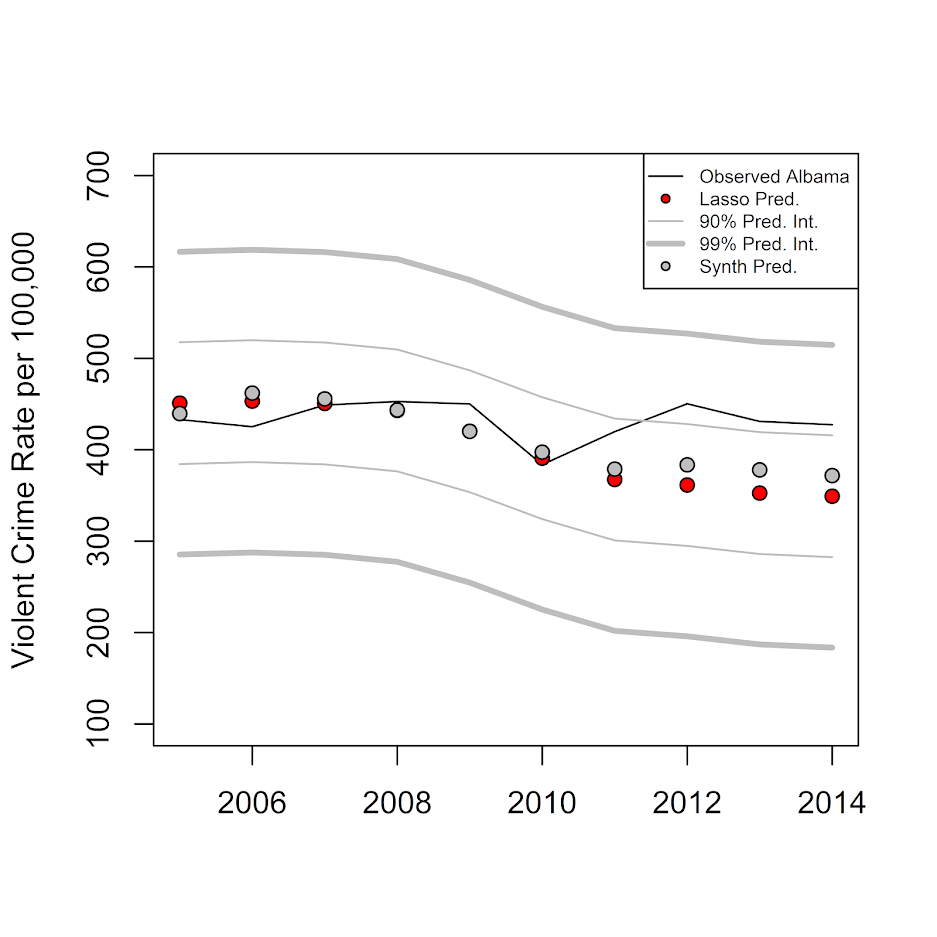

But when we look at variation in our placebo results (thin, purple lines), they are much wider than our conformal prediction intervals.

plot(wide_post[,1],wide_post[,2]-post_pred,type='l',ylim=c(-500,500),xlab='',ylab='Observed - Predicted (Violent Crime Rates)')
points(wide_post[,1],post_pred-post_pred,bg='red',pch=21)
lines(wide_post[,1],limits_01$lo-post_pred,col='grey',lwd=3)
lines(wide_post[,1],limits_01$up-post_pred,col='grey',lwd=3)

for (i in 2:ncol(PredRecent)){
  lines(wide_post[,1],DiffRecent[,i],col='#9400D340',lwd=0.5)
}

legend(x=2005.5,y=-700,legend=c("Observed Albama","Lasso Pred.","99% Pred. Int.","Placebos"),
       col=c("black","black","grey",'#9400D3'), pt.bg=c(NA,"red",NA,NA), lty=c(1,NA,1,1), 
       pch=c(NA,21,NA,NA), lwd=c(1,1,3,0.5), xpd=TRUE, horiz=TRUE, cex = 0.45)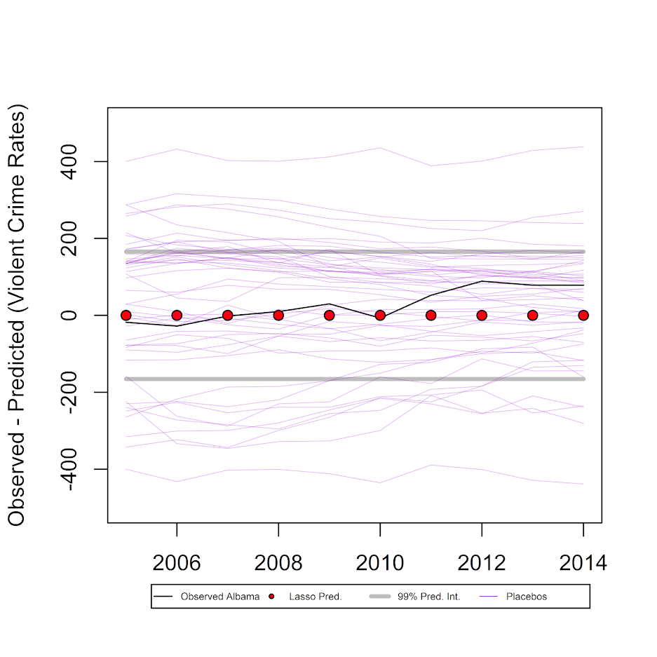

So I was hoping they would be the same (conformal would cover the placebo at the expected rate), but alas they are not. So I’m not sure if my conformal intervals are too small, or the placebo checks are extra noisy. I can’t prove it, but I suspect the placebo checks are somewhat noisy, mainly because there will always be some intervention that is idiosyncratic to specific donors over long periods of time that makes them no longer good counterfactuals. This seems especially true if you consider predictions further out from the treatment year. Although I find the logic of the placebo checks pretty convincing, so I am somewhat torn.

Since we have in this example 49 donors, the two-tailed p-value for being outside the placebos would be 2/(49+1)=0.04. Here we would need an intervention that either increased violent crime rates by plus/minus 400 per 100,000, pretty much an impossible standard given a baseline of only 400 crimes per 100,000 as of 2004. The 99% conformal intervals are still pretty wide, with an increase/decrease of about 150 violent crimes per 100,000 needed to be a significant change. The two lines way outside 400 happen to be Alaska and Wyoming, not DC, so maybe a tiny population state results in higher volatility problem. But besides them there are a bunch of placebo states around plus/minus 300 as well.

So caveat emptor if you want to use this idea in your own work, I don’t know if my suggestion is good or bad. Here it suggests its more diagnostic (smaller intervals) than the placebo checks, and isn’t limited by the number of potential donors in setting the alpha level for your tests (e.g. if you only have 10 potential donors your placebo checks are only 90% intervals).

Since this is just one example, there are a few things I would need to know before recommending it more generally. One is that it may not work with smaller pre time series and/or a smaller donor pool. (Not sure of any better way of checking than via a ton of different simulations.)

More general notes

Doing some more lit review while preparing this post, I appear to be like 15th in line to suggest this approach (so don’t take it as novel). In terms of using the lasso to estimate the synth weights, it seems Susan Athey and colleagues proposed something similar in addition to using other machine learning techniques. Also see Amjad et al. 2018 in the Journal of Machine Learning, and this workshop by Alex Hollingsworth and Coady Wing. I am not even the first one to think to use conformal prediction intervals apparently, see this working paper (Chernozhukov, Wuthrich, and Zhu, 2019) posted just a few weeks prior.

There is another R package, gsynth, that appears to solve the problem of p > n via a variable reduction technique (Xu, 2017). Xu also discusses how incorporating more information is really making different identification assumptions. So again just getting good predictions/minimizing the in-sample mean square error is not necessarily the right approach to get correct causal inferences.

Just a blog post, so again can’t say if this is an improvement over other work offhand. This is just illustrative that the bounds for the conformal prediction may be smaller than the typical permutation based approach. Casting it as a regression problem I intuitively grok more, and think opens up more possibilities. For example, you may want to use binomial logistic models instead of linear for the fitting process (so takes into account more volatility for smaller population states).