Repeating Charts in SPSS for unique IDs

The title is probably not that clear, but I’ve seen this request a few times and have used this trick in one my projects, so figured it would be a worthwhile topic to illustrate. So the problem is you have a background distribution, and you want to tailor a set of individual charts showing the unique individuals score against the background distribution. See two examples (1,2) of this question. In the first link I showed how one can do this by artificially duplicating the data in a specific way using VARSTOCASES and then using SPLIT FILE to generate the separate charts. Here I will show a python based solution that does not require duplicating the data.

So first we will start off with a set of fake student scores, 20 students with 5 scores each.

*Create some fake data, student test scores.
SET SEED 10.
INPUT PROGRAM.
STRING Student (A1).
LOOP #i = 1 TO 5.
  LOOP #j = 1 TO 20.
    COMPUTE Student = STRING(#j+64,PIB).
    COMPUTE Score = RND(RV.NORMAL(100,10)).
    END CASE.
  END LOOP.
END LOOP.
END FILE.
END INPUT PROGRAM.
DATASET NAME Student_Scores.
FORMATS Score (F3.0).
EXECUTE.

Now the students are listed as strings, but here I am going to use AUTORECODE to automatically turn the strings into number variables, and more importantly for what follows create a set of value labels corresponding to those unique strings.

*Use Auto-recode to make the variables 1 to N.
AUTORECODE VARIABLES = Student /INTO Student_N.
FORMATS Student_N (F6.0).

Now the workflow I want to do is to make a set of charts with the background a boxplot for the whole class, and then the individual students scores as foreground dots. To do this I will make a second set of scores that are missing for everyone except that one particular student, the specify MISSING=VARIABLEWISE on the GGRAPH command, and then superimpose Score2 over the boxplot of Score.

*Example of Individual chart.
NUMERIC flag (F1.0) Score2 (F3.0).

DO IF Student_N = 1.
  COMPUTE Score2 = Score.
  COMPUTE flag = 1.
ELSE.
  COMPUTE Score2 = $SYSMIS.
  COMPUTE flag = 0.
END IF.

GGRAPH
  /GRAPHDATASET NAME="graphdataset" VARIABLES=Score Score2 flag MISSING = VARIABLEWISE
  /GRAPHSPEC SOURCE=INLINE.
BEGIN GPL
  SOURCE: s=userSource(id("graphdataset"))
  DATA: Score=col(source(s), name("Score"))
  DATA: Score2=col(source(s), name("Score2"))
  COORD: rect(dim(1), transpose())
  GUIDE: axis(dim(1), label("Score"))
  GUIDE: legend(aesthetic(aesthetic.visible), null())
  GUIDE: text.title(label("Student: A"))
  ELEMENT: schema(position(bin.quantile.letter(Score)), color.interior(color.grey))
  ELEMENT: point.dodge.symmetric(position(bin.dot(Score2)), color.interior(color.red))
END GPL.
*cleaing up temp variables.
MATCH FILES FILE = * /DROP flag Score2.
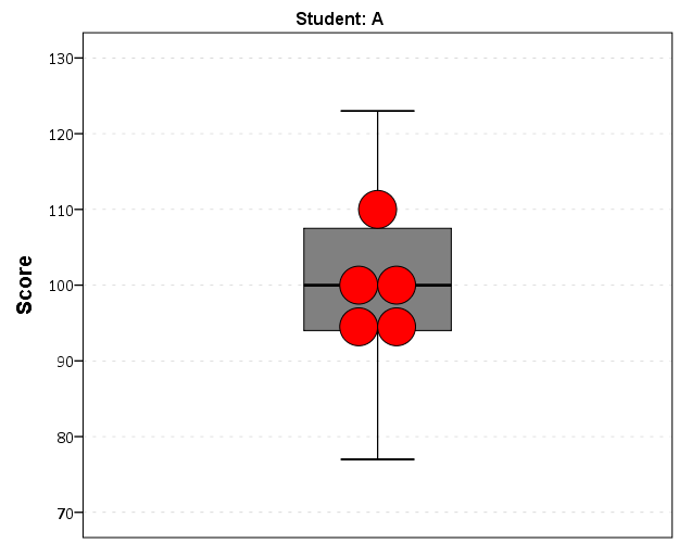
There are other ways to do this, like using the visible option in GPL aesthetics, but I don’t do that here because they still exist in the chart but simply aren’t shown. This causes problems with the dodging, and if you sent the chart in vector format the information would still be contained in the chart (e.g. if you need to aggregate the background data to be obfuscated for confidentiality reasons you don’t want it in the chart even if it is invisible). Here even the outlier dots in the boxplot are potentially disseminating confidential information, but for simplicity I don’t worry about that here (my syntax at the developerworks forum showed how you can build your own boxplot without having the points, it would be nice to have a no points option for the schema element).

So now the problem is looping through all of the individual students and generating a chart for each one. That is where the AUTORECODE comes in handy. I can grab all of the value labels from the SPSS dictionary and place them in a Python dictionary.

*Python to grab the different students.
BEGIN PROGRAM Python.
import spss
spss.StartDataStep()
datasetObj = spss.Dataset()
StudentLab = datasetObj.varlist['Student_N'].valueLabels
print StudentLab #this is a dictionary of all the unique students
spss.EndDataStep()
END PROGRAM.

Now with the StudentLab Python dictionary I can loop over the dictionary and submit the SPSS syntax for each unique student (using spss.Submit) using string substitutions. I first create the variables and set there formats outside of the loop (the chart inherits the formats). Then I just set several aesthetics of the charts so they are the same for every chart, e.g. the scale goes between 60 and 150, and the size of the superimposed points is 12.

*Now loop through the students.
OUTPUT CLOSE ALL.
BEGIN PROGRAM Python.
spss.Submit("NUMERIC flag (F1.0) Score2 (F3.0).")
for val, lab in StudentLab.data.iteritems():
  spss.Submit("""*Individual score chart.
DO IF Student_N = %d.
  COMPUTE Score2 = Score.
  COMPUTE flag = 1.
ELSE.
  COMPUTE Score2 = $SYSMIS.
  COMPUTE flag = 0.
END IF.
GGRAPH
  /GRAPHDATASET NAME="graphdataset" VARIABLES=Score Score2 flag MISSING = VARIABLEWISE
  /GRAPHSPEC SOURCE=INLINE.
BEGIN GPL
  SOURCE: s=userSource(id("graphdataset"))
  DATA: Score=col(source(s), name("Score"))
  DATA: Score2=col(source(s), name("Score2"))
  DATA: id=col(source(s), name("$CASENUM"), unit.category())
  DATA: flag=col(source(s), name("flag"), unit.category())
  COORD: rect(dim(1), transpose())
  GUIDE: axis(dim(1), label("Score"), delta(10), start(60))
  GUIDE: text.title(label("Student: %s"))
  GUIDE: legend(aesthetic(aesthetic.visible), null())
  SCALE: linear(dim(1), min(60), max(150))
  ELEMENT: schema(position(bin.quantile.letter(Score)), color.interior(color.grey))
  ELEMENT: point.dodge.symmetric(position(bin.dot(Score2)), color.interior(color.red),
           size(size."12"))
END GPL.
""" %(val,lab))
END PROGRAM.

I wanted to export these charts in the loop with the students names, using something like:

SpssOutputDoc.SelectLastOutput() #grab last output
SpssOutputDoc.ExportCharts(SpssClient.SpssExportSubset.SpssSelected, path + lab, SpssClient.ChartExportFormat.png)

but what happens with this is that it is always one behind (e.g. the first chart is selected in the second loop iteration). So what I did was to stuff all of the charts within a list and then loop over that list, select the chart, and then export it using SpssOutputDoc.ExportCharts (another option would be to use EXPORT OUTPUT and then either delete the output in-between charts or clear it, I wish OMS could export only charts). This would be more annoying with multiple individual charts, and could likely be made more concise, but here it is.

*Now exporting the individual charts.
BEGIN PROGRAM Python.
import SpssClient
SpssClient.StartClient()
SpssOutputDoc = SpssClient.GetDesignatedOutputDoc()

#creating a list of all the charts
OutputItems = SpssOutputDoc.GetOutputItems()
Charts = []
for index in range(OutputItems.Size()):
  OutputItem = OutputItems.GetItemAt(index)
  if OutputItem.GetType() == SpssClient.OutputItemType.CHART:
    Charts.append(OutputItem)

labList = []
for val, lab in StudentLab.data.iteritems():
  labList.append(lab)

path = "C:/Users/andrew.wheeler/Dropbox/Documents/BLOG/RepeatingCharts/"

for chart,lab in zip(Charts,labList):
  SpssOutputDoc.ClearSelection() #clear prior selections
  chart.SetSelected(True) #select chart
  #export chart
  SpssOutputDoc.ExportCharts(SpssClient.SpssExportSubset.SpssSelected, path + lab, SpssClient.ChartExportFormat.png)
END PROGRAM.

Here is a screen shot of the resulting images in my folder.

So this will export the charts to PNG format with the image name the same as the students in the file (so the name needs to be in a format appropriate to save a file name). Annoyingly SPSS appends 1 to the end of all charts, even if it is only exporting one chart. Here is an example of the student G’s chart.

Eventually I will figure out how to send emails via Python, and this would be a good tool for individualized report cards for a class. Here is a copy of the full syntax to more easily run on your local machine (just replace path with a location on your local machine).

Turning data from Python into SPSS data

I’ve shown how you can grab data from SPSS and use it in Python commands, and I figured a post about the opposite process (taking data in Python and turning it into an SPSS data file) would be useful. A few different motivating examples are:

So first as a simple illustration, lets make a set of simple data in Python as a list of lists.

BEGIN PROGRAM Python.
MyData = [(1,2,'A'),(4,5,'B'),(7,8,'C')]
END PROGRAM.

Now to export this data into SPSS you can use spss.StartDataStep(), append variables using varlist.append and then add cases using cases.append (see the Python programming PDF that comes with SPSS in the help to peruse all of these functions plus the documentation). This particular codes adds in 3 variables (two numeric and one string) and then loops through the data python object and adds those cases to the define SPSS dataset.

BEGIN PROGRAM Python.
import spss
spss.StartDataStep()                   #start the data setp
MyDatasetObj = spss.Dataset(name=None) #define the data object
MyDatasetObj.varlist.append('X1',0)    #add in 3 variables
MyDatasetObj.varlist.append('X2',0)
MyDatasetObj.varlist.append('X3',1)
for i in MyData:                       #add cases in a loop
  MyDatasetObj.cases.append(i)
spss.EndDataStep()
END PROGRAM.

Here this will create a SPSS dataset and give it a generic name of the form xDataset? where ? will be an incrementing number based on the session history of naming datasets. To specify the name beforehand you need to use the SPSS command DATASET DECLARE X. and then place the dataset name as the option in the spss.Dataset(name='X') command.

As linked above I have had to do this a few times from Python objects, so I decided to make a bit of a simpler SPSS function to take care of this work for me.

BEGIN PROGRAM Python.
#Export to SPSS dataset function
import spss

def SPSSData(data,vars,types,name=None):
  VarDict = zip(vars,types) #combining variables and 
                            #formats into tuples
  spss.StartDataStep()
  datasetObj = spss.Dataset(name=name) #if you give a name, 
                                       #needs to be declared
  #appending variables to dataset
  for i in VarDict:
    datasetObj.varlist.append(i[0],i[1])
  #now the data
  for j in data:
    datasetObj.cases.append(list(j))
  spss.EndDataStep()
END PROGRAM.

This code takes an arbitrary Python object (data), and two lists, one of the SPSS variable names and the other of the format for the SPSS variables (either 0 for numeric or an integer for the size of the strings). To transform the data to SPSS, it needs a list of the same dimension as the variables you have defined, so this works for any data object that can be iterated over and that can be coerced to returning a list. Or more simply, if list(data[0]) returns a list of the same dimensions for the variables you defined, you can pass the data object to this function. This won’t work for all situations, but will for quite a few.

So with the permutation examples I previously linked to, we can use the itertools library to create a set of all the different permutations of string ABC. Then I define a set of variables and formats as lists, and then we can use the SPSSData function I created to make a new dataset.

DATASET DECLARE Combo.
BEGIN PROGRAM Python.
import itertools
YourSet = 'ABC' 
YourLen = 3
x = itertools.permutations(YourSet,YourLen)
v = ['X1','X2','X3']
t = [1,1,1]
SPSSData(data=x,vars=v,types=t,name='Combo')
END PROGRAM. 

This work flow is not optimal if you are creating the data in a loop (such as in the Google Places API example I linked to earlier), but works well for static python objects, such as the object returned by itertools.

Using regular expressions in SPSS

SPSS has a native set of string manipulations that will suffice for many simple situations. But with the ability to call Python routines, one can use regular expressions (or regex is often used for short) to accomplish more complicated searches. A post on Nabble recently discussed extracting zip codes from address data as an example, and I figured it would be a good general example for the blog.

So first, the SPSSINC TRANS command basically allows you to use Python functions the same as SPSS functions to manipulate a set of data. So for example if there is a function in Python and it takes one parameter, say f(a), and returns one value, you can use SPSSINC TRANS to have SPSS return a new variable based on this Python function. So say we have a variable named X1 and we want to get the result of f(X1) for every case in our dataset, as long as the function f() is available in the Python environment the following code would accomplish this:

SPSSINC TRANS RESULT=f_X TYPE=0 /FORMULA f(X1).

This will create a new variable in the active SPSS dataset, f_X, that is the result based on passing the values of X1 to the function. The TYPE parameter specifies the format of the resulting variable; 0 signifies that the result of the function is a number and if it is a string you simply pass the size of the string.

So using SPSSINC TRANS, we can create a function that does a regular expression search and returns the matching substring. The case on Nabble is a perfect example, extracting a set of 5 consecutive digits in a string, that is difficult to do with native SPSS string manipulation functions. It is really easy to do with regex’s though.

So the workflow is quite simple, import the re library, define your regular expression search, and then make your function. For SPSS if you return more than one value for a function in expects it is a tuple. If you look at the Nabble thread it discusses more complicated regex’s but here I keep it simple, \d{5}. This is interpreted as search for \d, which is shorthand for all digits 0-9, and then {n} is shorthand for search for the preceding string n times in a row.

BEGIN PROGRAM Python.
import re
s = re.compile(r'\d{5}')
def SearchZip(MyStr):
  Zip = re.search(s,MyStr)
  if Zip:
    return [Zip.group()]
  else:
    return [""]
END PROGRAM. 

Lets make up some test data to test our function within Python to make sure it works correctly.

BEGIN PROGRAM Python. 
#Lets try a couple of examples. 
test = ["5678 maple lane townname, md 20111", 
        "123 oak st #4 someplace, RI 02913-1234", 
        "9011 cedar place villagename"] 

for i in test: 
  print i 
  print SearchZip(i) 
END PROGRAM. 

And this outputs in the SPSS window:

5678 maple lane townname, md 20111 
['20111'] 
123 oak st #4 someplace, RI 02913-1234 
['02913'] 
9011 cedar place villagename 
['']

So at this point it is as simple as below (assuming Address is the string field in the SPSS dataset we are searching):

SPSSINC TRANS RESULT=Zip TYPE=5 /FORMULA SearchZip(Address).

This just scratches the surface of what regex’s can do. Based on some of the back and forth on the recent Nabble discussion this is a pretty general solution that searches an address at the end of the string, optionally finds a dash or a space, and then searches for 4 digits, re.compile(r"(\d{5})(?:[\s-])?(\d{4})?\s*$"). Note because the middle grouping is optional this would match 9 digits in a row (which I think is ok in my experience cleaning string address fields, especially since the search is limited to the end of the string).

Here is the full function for use. Note if you get errors about the None type conversion update your version of SPSSINC TRANS, see this Nabble thread for details.

BEGIN PROGRAM Python.
import re
SearchZ = re.compile(r"(\d{5})(?:[\s-])?(\d{4})?\s*$") #5 digits in a row @ end of string
                                                       #and optionally space or dash plus 4 digits
def SearchZip(MyStr):
  Zip = re.search(SearchZ,MyStr)
  #these return None if there is no match, so just replacing with
  #a tuple of two None's if no match
  if Zip:
    return Zip.groups()
  else:
    return (None,None)

#Lets try a couple of examples. 
test = ["5678 maple lane townname, md 20111", 
        "5678 maple lane townname, md 20111 \t",
        "123 oak st #4 someplace, RI 02913-1234", 
        "9011 cedar place villagename",
        "123 oak st #4 someplace, RI 029131234",
        "123 oak st #4 someplace, RI 02913 1234"] 

for i in test: 
  print [i] 
  print SearchZip(i) 
END PROGRAM. 

Because this returns two separate groups, the SPSSINC TRANS command will need to specify multiple variables, so would be something like:

SPSSINC TRANS RESULT=Zip5 Zip4 TYPE=5 4 /FORMULA SearchZip(Address).

Estimating group based trajectory models using SPSS and R

For a project I have been estimating group based trajectory models for counts of crime at micro places. Synonymous with the trajectory models David Weisburd and colleagues estimated for street segments in Seattle. Here I will show how using SPSS and the R package crimCV one can estimate similar group based trajectory models. Here is the crimCV package help and here is a working paper by the authors on the methodology. The package specifically estimates a zero inflated poisson model with the options to make the 0-1 part and/or the count part have quadratic or cubic terms – and of course allows you specify the number of mixture groups to search for.

So first lets make a small set of fake data to work with. I will make 100 observations with 5 time points. The trajectories are three separate groups (with no zero inflation).

*Make Fake data.
SET SEED 10.
INPUT PROGRAM.
LOOP Id = 1 TO 100.
END CASE.
END LOOP.
END FILE.
END INPUT PROGRAM.
DATASET NAME OrigData.
*Make 3 fake trajectory profiles.
VECTOR Count(5,F3.0).
DO REPEAT Count = Count1 TO Count5 /#iter = 1 TO 5.
COMPUTE #i = #iter - 3.
COMPUTE #ii  = #i**2.
COMPUTE #iii = #i**3.
  DO IF Id <= 30.
    COMPUTE #P    = 10 + #i*0.3 + #ii*-0.1 + #iii*0.05.
    COMPUTE Count = RV.POISSON(#P).
  ELSE IF Id <=60.
    COMPUTE #P    =  5 + #i*-0.8 + #ii*0.3 + #iii*0.05.
    COMPUTE Count = RV.POISSON(#P).
  ELSE. 
    COMPUTE #P    =  4 + #i*0.8 + #ii*-0.5 + #iii*0.
    COMPUTE Count = RV.POISSON(#P).
  END IF.
END REPEAT.
FORMATS Id Count1 TO Count5 (F3.0).
EXECUTE.

Note The crimCV package wants the data to be wide format for the models, that is each separate time point in its own column. Now we can call R code using BEGIN PROGRAM R to recreate the wide SPSS dataset in an R data frame.

*Recreate SPSS data in R data frame.
BEGIN PROGRAM R.
casedata <- spssdata.GetDataFromSPSS(variables=c("Id","Count1","Count2",
                                                "Count3","Count4","Count5")) #grab data from SPSS
casedataMat <- as.matrix(casedata[,2:6]) #turn into matrix
#summary(casedata) #check contents
#casedataMat[1:10,1:5]
END PROGRAM.

Now to fit one model with 3 groups (without calculating the cross validation statistics) the code would be as simple as:

*Example estimating model with 3 groups and no CV.
BEGIN PROGRAM R.
library(crimCV)
crimCV(casedataMat,3,rcv=FALSE,dpolyp=3,dpolyl=3)
END PROGRAM.

But when we are estimating these group based trajectory models we don’t know the number of groups in advance. So typically one progressively fits more groups and then uses model selection criteria to pick the mixture solution that best fits the data. Here is a loop I created to successively estimate models with more groups and stuffs the models results in a list. It also makes a separate data frame that saves the model fit statistics, so you can see which solution fits the best (at least based on these statistics). Here I loop through estimates of 1 through 4 groups (this takes about 2 minutes in this example). Be warned – here are some bad programming practices in R (the for loops are defensible, but growing the lists within the loop is not – they are small though in my application and I am lazy).

*looping through models 1 through 4.
BEGIN PROGRAM R.
results <- c()  #initializing a set of empty lists to store the seperate models
measures <- data.frame(cbind(groups=c(),llike=c(),AIC=c(),BIC=c(),CVE=c())) #nicer dataframe to check out model 
                                                                            #model selection diagnostics
max <- 4 #this is the number of grouping solutions to check

#looping through models
for (i in 1:max){
    model <- crimCV(casedataMat,i,rcv=TRUE,dpolyp=3,dpolyl=3)
    results <- c(results, list(model))
    measures <- rbind(measures,data.frame(cbind(groups=i,llike=model$llike,
                                          AIC=model$AIC,BIC=model$BIC,CVE=model$cv)))
    #save(measures,results,file=paste0("Traj",as.character(i),".RData")) #save result
    }
#table of the model results
measures
END PROGRAM.

In my actual application the groups take a long time to estimate, so I have the commented line saving the resulting list in a file. Also if the model does not converge it breaks the loop. So here we see that the mixture with 3 groups is the best fit according to the CVE error, but the 2 group solution would be chosen by AIC or BIC criteria. Just for this tutorial I will stick with the 3 group solution. We can plot the predicted trajectories right within R by selecting the nested list.

*plot best fitting model.
BEGIN PROGRAM R.
plot(results[[3]])
#getAnywhere(plot.dmZIPt) #this is the underlying code
END PROGRAM.

Now the particular object that stores the probabilities is within the gwt attribute, so we can transform this to a data frame, merge in the unique identifier, and then use the STATS GET R command to grab the resulting R data frame back into an SPSS dataset.

*Grab probabiltiies back SPSS dataset.
BEGIN PROGRAM R.
myModel <- results[[3]] #grab model
myDF <- data.frame(myModel$gwt) #probabilites into dataframe
myDF$Id <- casedata$Id #add in Id
END PROGRAM.
*back into SPSS dataset.
STATS GET R FILE=* /GET DATAFRAME=myDF DATASET=TrajProb.

Then we can merge this R data frame into SPSS. After that, we can classify the observations into groups based on the maximum posterior probability of belonging to a particular group.

*Merge into original dataset, and the assign groups.
DATASET ACTIVATE OrigData.
MATCH FILES FILE = *
  /FILE = 'TrajProb'
  /BY ID
  /DROP row.names.
DATASET CLOSE TrajProb.
*Assign group based on highest prob.
*If tied last group wins.
VECTOR X = X1 TO X3.
COMPUTE #MaxProb = MAX(X1 TO X3).
LOOP #i = 1 TO 3.
  IF X(#i) = #MaxProb Group = #i.
END LOOP.
FORMATS Group (F1.0).

Part of the motivation for doing this is not only to replicate some of the work of Weisburd and company, but that it has utility for identifying long term hot spots. Part of what Weisburd (and similarly I am) finding is that crime at small places is pretty stable over long periods of time. So we don’t need to make up to date hotspots to allocate police resources, but are probably better off looking at crime over much longer periods to identify places for targeted strategies. Trajectory models are a great tool to help identify those long term high crime places, same as geographic clustering is a great tool to help identify crime hot spots.

Aggregating values in time series charts

One common task I undertake in is to make time series graphs of crime counts, often over months or shorter time periods. Here is some example data to illustrate, a set of 20 crimes with a particular date in 2013.

*Make some fake data.
SET SEED 10.
INPUT PROGRAM.
LOOP #i = 1 TO 20.
  COMPUTE #R = RV.UNIFORM(0,364).
  COMPUTE DateRob = DATESUM(DATE.MDY(1,1,2013),#R,"DAYS").
  END CASE.
END LOOP.
END FILE.
END INPUT PROGRAM.
FORMATS DateRob (ADATE10).
EXECUTE.

SPSS has some convenient functions to aggregate right within GGRAPH, so if I want a chart of the number of crimes per month I can create my own Month variable and aggregate. The pasted GGRAPH code is generated directly though the Chart Builder GUI.

COMPUTE Month = XDATE.MONTH(DateRob).
FORMATS Month (F2.0).

*Default Line chart.
GGRAPH
  /GRAPHDATASET NAME="graphdataset" VARIABLES=Month COUNT()[name="COUNT"] MISSING=LISTWISE 
    REPORTMISSING=NO
  /GRAPHSPEC SOURCE=INLINE.
BEGIN GPL
  SOURCE: s=userSource(id("graphdataset"))
  DATA: Month=col(source(s), name("Month"), unit.category())
  DATA: COUNT=col(source(s), name("COUNT"))
  GUIDE: axis(dim(1), label("Month"))
  GUIDE: axis(dim(2), label("Count"))
  SCALE: linear(dim(2), include(0))
  ELEMENT: line(position(Month*COUNT), missing.wings())
END GPL.

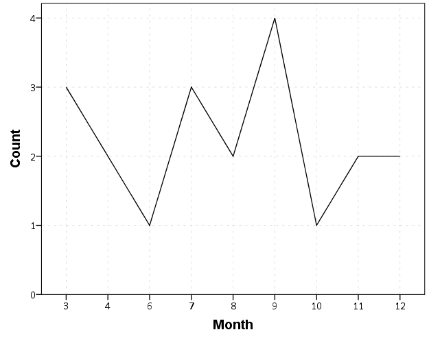
So at first glance that looks alright, but notice that the month’s do not start until 3. Also if you look close you will see a 5 is missing. What happens is that to conduct the aggregation in GGRAPH, SPSS needs to treat Month as a categorical variable – not a continuous one. SPSS only knows of the existence of categories contained in the data. (A similar thing happens in GROUP BY statements in SQL.) So SPSS just omits those categories.

We can manually specify all of the month categories in the axis. To reinforce where the measurements come from I also plot the points on top of the line.

*Line chart with points easier to see.
GGRAPH
  /GRAPHDATASET NAME="graphdataset" VARIABLES=Month COUNT()[name="COUNT"] MISSING=LISTWISE 
    REPORTMISSING=NO
  /GRAPHSPEC SOURCE=INLINE.
BEGIN GPL
  SOURCE: s=userSource(id("graphdataset"))
  DATA: Month=col(source(s), name("Month"), unit.category())
  DATA: COUNT=col(source(s), name("COUNT"))
  GUIDE: axis(dim(1), label("Month"))
  GUIDE: axis(dim(2), label("Count of Robberies"))
  SCALE: cat(dim(1), include("1","2","3","4","5","6","7","8","9","10","11","12"))
  SCALE: linear(dim(2), include(0))
  ELEMENT: line(position(Month*COUNT), missing.wings())
  ELEMENT: point(position(Month*COUNT), color.interior(color.black), 
           color.exterior(color.white), size(size."10"))
END GPL.

So you can see that include statement with all of the month numbers. You can also see what that mysterious missing.wings() function actually does in this example. It is misleading though, as 5 isn’t missing, it is simply zero.

A simple workaround for this example is to just use a bar chart. A zero bar is not misleading.

GGRAPH
  /GRAPHDATASET NAME="graphdataset" VARIABLES=Month COUNT()[name="COUNT"] MISSING=LISTWISE 
    REPORTMISSING=NO
  /GRAPHSPEC SOURCE=INLINE.
BEGIN GPL
  SOURCE: s=userSource(id("graphdataset"))
  DATA: Month=col(source(s), name("Month"), unit.category())
  DATA: COUNT=col(source(s), name("COUNT"))
  GUIDE: axis(dim(1), label("Month"))
  GUIDE: axis(dim(2), label("Count of Robberies"))
  SCALE: cat(dim(1), include("1","2","3","4","5","6","7","8","9","10","11","12"))
  SCALE: linear(dim(2), include(0))
  ELEMENT: interval(position(Month*COUNT))
END GPL.

I often prefer line charts for several reasons though, often to superimpose multiple lines (e.g. I may want to put the lines for counts of crimes in 2012 and 2011 as well). Line charts are clearly superior to clustered bar charts in that situation. Also I prefer to be able to keep time is a numerical variable in the charts, and one can’t do that with aggregation in GGRAPH.

So I do the aggregation myself.

*Make a new dataset.
DATASET DECLARE AggRob.
AGGREGATE OUTFILE='AggRob'
  /BREAK = Month
  /CountRob = N.
DATASET ACTIVATE AggRob.

But we have the same problem here, in that months with zero counts are not in the data. To fill in the zeroes, I typically make a new dataset of the date ranges using INPUT PROGRAM and loops, same as I did to make the fake data at the beginning of the post.

*Make a new dataset to expand to missing months.
INPUT PROGRAM.
LOOP #i = 1 TO 12.
  COMPUTE Month = #i.
  END CASE.
END LOOP.
END FILE.
END INPUT PROGRAM.
DATASET NAME TempMonExpan.

Now we can simply merge this expanded dataset back into AggRob, and the recode the system missing values to zero.

*File merge back into AggRob.
DATASET ACTIVATE AggRob.
MATCH FILES FILE = *
  /FILE = 'TempMonExpan'
  /BY Month.
DATASET CLOSE TempMonExpan.
RECODE CountRob (SYSMIS = 0).

Now we can make our nice line chart with the zeros in place.

GGRAPH
  /GRAPHDATASET NAME="graphdataset" VARIABLES=Month CountRob
  /GRAPHSPEC SOURCE=INLINE.
BEGIN GPL
  SOURCE: s=userSource(id("graphdataset"))
  DATA: Month=col(source(s), name("Month"))
  DATA: CountRob=col(source(s), name("CountRob"))
  GUIDE: axis(dim(1), label("Month"), delta(1), start(1))
  GUIDE: axis(dim(2), label("Count of Robberies"), start(0))
  SCALE: linear(dim(1), min(1), max(12))
  SCALE: linear(dim(2), min(-0.5))
  ELEMENT: line(position(Month*CountRob))
  ELEMENT: point(position(Month*CountRob), color.interior(color.black), 
           color.exterior(color.white), size(size."10"))
END GPL.

To ease making these separate time series datasets I have made a set of macros, one named !TimeExpand and the other named !DateExpand. Both take a begin and end date and then make an expanded dataset of times. The difference between the two is that !TimeExpand takes a user specified step size, and !DateExpand takes a string of the types used in SPSS date time calculations. The situation in which I like to use !TimeExpand is when I do weekly aggregations from a specified start time (e.g. the weeks don’t start over at the beginning of the year). It also works for irregular times though, say if you wanted 15 minute bins. !DateExpand can take years, quarters, months, weeks, days, hours, minutes, and seconds. The end dates can also be system variables like $TIME as well. The macro can be found here, and it contains several examples within. Update: I have added a few macros that do the same thing for panel data. It just needs to take one numeric variable as the panel id, otherwise the argument for the macros are the same.

Using Python to geocode data in SPSS

This is the first time since I’ve been using SPSS that I have regular access to Python and R programmability in all of the different places I use SPSS (home and multiple work computers). So I’ve been exploring more solutions to use these tools in regular data analysis and work-flows – of course to accomplish things that can not be done directly in native SPSS code.

The example I am going to show today is using geopy, a Python library that places several geocoding API’s all in a convenient set of scripts. So first once geopy is installed you can call Python code within SPSS by placing it within a BEGIN PROGRAM and END PROGRAM blocks. Here is an example modified from geopy’s tutorial.


BEGIN PROGRAM.
from geopy import geocoders
g = geocoders.GoogleV3()
place, (lat, lng) = g.geocode("135 Western Ave. Albany, NY")  
a = [place, lat, lng]
print a
END PROGRAM.

Now what we want to do is to geocode some address data that is currently stored in SPSS case data. So here is an example dataset with some addresses in Albany.


DATA LIST LIST ("|") / Address (A100).
BEGIN DATA
135 Western Ave. Albany, NY
Western Ave. and Quail St Albany, NY
325 Western Ave. Albany, NY
END DATA.
DATASET NAME Add.

Here I will use the handy SPSSINC TRANS function (provided when installing Python programmability – and as of SPSS 22 installed by default with SPSS) to return the geocoded coordinates using the Google API. The geocode function from geopy does not return the data in an array exactly how I want it, so what I do is create my own function, named g, and it coerces the individual objects (place, lat and lng) into an array and returns that.


BEGIN PROGRAM.
from geopy import geocoders
def g(a):
  g = geocoders.GoogleV3()
  place, (lat, lng) = g.geocode(a)
  return [place, lat, lng]
print g("135 Western Ave. Albany, NY")
END PROGRAM.

Now I can use the SPSSINC TRANS function to return the associated place string, as well as the latitude and longitude coordinates from Google.


SPSSINC TRANS RESULT=Place Lat Lng TYPE=100 0 0
  /FORMULA g(Address).

Pretty easy. Note that (I believe) the Google geocoding API has a limit of 2,500 cases – so don’t go submitting a million cases to be geocoded (use an offline solution for that). Also a mandatory mention should be made of the variable reliability of online geocoding services.

Working with American Community Survey Data in SPSS

Going through the documentation and downloading data from the Census is quite a chore. Here I am going to give some example SPSS functions I have created for working with the plain text 5 year summary files available from the Census’s FTP site. I mainly use this for mapping purposes, in particular mapping the small area census geographies. Here I have posted the code used for this analysis.

To start off, last time I checked you can not get block group data from the Census’s GUI interface that allows you to point and click certain data downloads, so if you want small geographies you have to grab it from the plain text files. Of course, if you check out the technical document you will see there are hundreds of tables which each have hundreds of variables. So if you navigate to Appendix E (page 45) of the Tech Doc. You will see here that a set of variables in a table, say table B01001 (which contains variables related to Sex by Age) is available at the block group level and is in the summary file sequence number 1.

Slightly confusingly, the sequence number is what signals which plain text file the data is located in, and if you download and uzip the state table you will see a set of text files that look like e20125ny0002000.txt or m20125ny0002000.txt. The e stands for estimates, and the m stands for margin of error. These comma separated files (with no text qualifiers, as they do not have strings with commas) contain a set of 6 consistent variables at the start, and then a variable number of variables at the end of the file. From here on when I refer to a table, I don’t mean the B01001 descriptor, I mean either the sequence number and/or the actual text file the data is located in.

Associating the particular variable in a table to its definition is accomplished with the sequence number and table number lookup file. I think I am just going to say look at my code on how to associate those two tables – I’m pretty sure anything I narrate will only confuse matters. Unfortunately the line number field does not correspond to the actual variable order in the text file – you have to take into account that the same text file contains multiple sequences of line numbers that restart at 1.

So again I have all of the materials I will use in the post available to download (linked earlier in the post), but to follow along with your own data you will need;

  • The ACS Technical Doc (to look up what variables you want).
  • The sequence number and table number lookup file (to figure out what the variables represent)
  • An unzipped file of the actual data
  • The SPSS MACRO to grab the ACS data (contained in the ACS_MACRO.sps file) and the VariableLabels.sps file that helps to figure out what the variables are.

Here I placed that and my syntax all into the same folder. So to reference these files I only need to define one file handle. So to start lets define a file handle named data and then insert my two other syntax files. The first grabs the sequence number table lookup (and names the SPSS dataset MetaACS) and does some data manipulations on that lookup table. The second INSERT command defines our macro to grab the actual ACS data. (You can open up the ACS_Examples.sps syntax to follow along – the example tables are for New York State block groups only file.)


FILE HANDLE data /name = "!Your file location Here!".
INSERT FILE = "data\VariableLabels.sps" CD=YES.
INSERT FILE = "data\ACS_MACRO.sps". 

So now from looking at the technical document I know I want to grab the information from the Sex by Age table. This happens to be sequence number 2. So first I run the command:


!ACSTable Seq = 2.

And this produces a table that looks like below:

In this table the TableTitle is the description of the variable, and the Order column tells you what number the variable is in the subsequent text file. Not all rows will refer to a variable, and so we see here that for the SEX BY AGE table (first row), for the subsequent variables, V1 is the Total population, V2 is the Male population, and V3 is the Male population Under 5 years of age. Most of the variables provided by the ACS have this subsequent nesting structure, and so although thousands of variables exist in all of the tables, they just tend to be various demographic breakdowns into more specific categories.

The variable in the right most column tells us that in this table (besides the 6 that are at the start of every table) there ends up being 235 total variables in the table. So now we can call the syntax to grab the actual data.


!ImportACS File = 'data\e20125ny0002000.txt' Table = T2 Cells = 235.

This !ImportACS macro takes as parameters:

  • File – the full file location (in quotes) of the text file that contains the data
  • Table – this token assigns the dataset name and the prefix for all of the variables in the file (excluding the 6 consistent ones). So it needs to follow the conventions for naming those files.
  • Cells – this defines the total number of variables that the table contains after the 6 consistent ones.

So after you run this syntax it will open a table that has the variables as below:

So we can see the variables FileID, Filetype, State, chariter, sequence, and LOGRECNO will always be the first six variables. After those we have a set of 235 variables of the form T2_1, T2_2 …. T2_235.

As I noted from the original !ACSTable macro, we can look up each individual value, and so we know T2_1 is the total population, T2_2 is the male population, and T2_3 is the male population under 5 years of age. So when I grabbed this table I actually wanted the entire population between 5 and 17 years old (not just males or females). So to calculate that variable I need to sum several variables together.


COMPUTE Under17 = SUM(T2_4 to T2_6,T2_28 to T2_30).

I have some further examples in the ACS_Example.sps syntax that grabs data on race, children in female headed households, Spanish speaking households, and households below poverty. I then merge the tables together using the LOGRECNO variable (which is the census geography id).

From this you can grab whatever tables you want and then merge them together. Digging through the documentation tends to be the hardest part, given how large it is. I originally wrote this for the 5 year estimates in 2010 and recently needed to revisit with 2012 data. The format of the data is the same, but the sequence numbers differed from 2010 to 2012. I only provide examples with the estimates data here, but the macro should work just fine with the margin of error data files as well.

Quick SPSS tip: Suppressing output

When running commands in SPSS, it routes summaries and output of particular functions to the active Output document. This is very nice for statistical reporting of various tables, like crosstabs or frequencies or nested regression models. This however is not so nice in some circumstances in which the tables are very big. Rendering the output of these large tables takes a fair bit of memory. Also it is near impossible to navigate the tables when they get very large. (I should note SPSS does have some nice pivot table functionality for nested tables, e.g. in CTABLES, but the examples that follow with don’t apply to that.)

A few examples I come across tables being annoying often are:

  • Large correlation matrices or distance matrices (which I often export directly to an SPSS file – note PROXIMITIES has the option to suppress the table on the command, CORRELATIONS does not).
  • Macro commands that have various data transformations and may produce a series of tables (e.g. VARSTOCASES or CREATE). The regression procedures tend to be the worst offenders, so if you say want the predicted values from a REGRESSION or covariances from FACTOR you get half a dozen other tables along with it.
  • Using SPLIT FILE with many groups.

There are basically two ways I know of to easily suppress the output:

  • Use the Output Management System (OMS)
  • Use SET RESULTS OFF ERRORS OFF. – Via David Marso

It is pretty simple to use either to just suppress the output. For OMS it would be:


OMS /SELECT ALL EXCEPT = [WARNINGS] 
    /DESTINATION VIEWER = NO 
    /TAG = 'NoJunk'.
*Your Commands here.
OMSEND TAG = 'NoJunk'.

The OMS command just grabs all output except for warnings and tells SPSS to not send it to the output viewer. Per some comments I updated the example to take a TAG subcommand on the OMS command, as this allows you to have multiple OMS statements and only turn off specific ones at a time. Here it is hard to see the utility, but it should be more obvious when we place this inside a macro.

To replace the OMS example with the SET RESULTS OFF ERRORS OFF. trick by David Marso, you would basically just replace the original OMS command and then wrap it in PRESERVE and RESTORE statements.


PRESERVE.
SET RESULTS OFF ERRORS OFF.
*Your Commands here.
RESTORE.

Because this changes the system output settings, it is always a good idea to use PRESERVE and then set the user settings back to what they originally were with RESTORE. OMS has the slight advantage here that you can set it to still print warning messages. (I do not know off-hand which version of SPSS the OMS command was introduced.)

I will give a pretty simple example of using OMS with CORRELATIONS to suppress such junk output. A question on SO the other day asked about producing all pair-wise correlations above a threshold, and I gave an answer and an example macro to accomplish this (FYI such things would be useful for producing corrgrams or a network diagram of correlations). The output in that example though still produces the correlation table (which in the original posters situation would produce a 200*200 table in the output) and will produce various junk when running the VARSTOCASES command. Here I wrap the macro in the OMS statement suppressing the tables and you do not get such junk.


DEFINE !CorrPairs (!POSITIONAL !CMDEND)
OMS /SELECT ALL EXCEPT = [WARNINGS] 
    /DESTINATION VIEWER = NO 
    /TAG = "CorrPairs".
DATASET DECLARE Corrs.
CORRELATIONS  /VARIABLES=!1  /MATRIX=OUT('Corrs'). 
DATASET ACTIVATE Corrs.
SELECT IF ROWTYPE_ = "CORR".
COMPUTE #iter = 0.
DO REPEAT X = !1.
  COMPUTE #iter = #iter + 1.
  IF #iter > ($casenum-1) X = $SYSMIS.
END REPEAT.
VARSTOCASES /MAKE Corr FROM !1 /INDEX X2 (Corr) /DROP ROWTYPE_.
RENAME VARIABLES (VARNAME_ = X1).
OMSEND TAG="CorrPairs".
!ENDDEFINE.

And now using the same example data as I used on the question:


***********************************.
*Making fake data.
set seed 5.
input program.
loop i = 1 to 100.
end case.
end loop.
end file.
end input program.
dataset name test.
compute #base = RV.NORMAL(0,1).
vector X(20).
loop #i = 1 to 20.
compute X(#i) = #base*(#i/20)  + RV.NORMAL(0,1).
end loop.
exe.
***********************************.
*Now generate correlation pairs.
!CorrPairs X1 to X20.

If you want to see all the output that was originally generated just comment out the two lines with the OMS and OMSEND statements in the macro. Newer versions of SPSS limit the number of rows displayed in output tables, so your system shouldn’t crash with newer versions of SPSS even when you have enormous tables. But the advice here still applies, as you might as well route the output for those large tables somewhere else so that they are easier to explore (either using OMS to save the tables or helper functions on certain commands to export tables).

Querying Graph Neighbors in SPSS

The other day I showed how one could make an edge list in SPSS, which is needed to generate network graphs. Today, I will show how one can use an edge list in long format to identify neighbors for higher degree relationships.

So to start, what do I mean by a neighbor of higher degree relationship? Lets say I have a relationship between two nodes A B. Now lets also say I have another relationship between nodes B C. I might say that A and C don’t have a direct relationship, but they are related in that they both have a relationship to B. So A is a first degree neighbor of B, and A is a second degree neighbor of C. If I drew a graph of the listed network, the degree relationship between A and C would be the minimum number of edges one would have to traverse to get from the A node to the C node.

A  B  C

Why would a criminologist or crime analyst care about relationships of higher degrees? Well, here are two examples I am familiar with in criminology;

For more simple and practical motivation for crime analysts, you may just have some particular individuals who you want to have targeted enforcement towards (known chronic offenders, violent gang members) and you would like to compile a more extended network of individuals related to those particular offenders to keep an eye on, or further investigate for possible ties to co-offending or gang activity.

So to start in SPSS, lets say that we have a edge list in long format, where there is a column that ID’s each person, and another column that shows if those two people are related at the same event. Exampe ties for a crime analyst may be victimizations, or co-offending, or being stopped for field interviews at the same time.

*Long dataset marking people sharing same incident (ID).
data list free / IncID (F2.0) Person (A15).
begin data
1 John 
1 Mary
2 John 
2 Frank
3 John 
3 William
4 John 
4 Andrew
5 Mary 
5 Frank
6 Mary 
6 William
7 Frank 
7 Kelly
8 Andrew 
8 Penny
9 Matt 
9 Andrew
10 Kelly 
10 Andrew
end data.
dataset name long.
dataset activate long.

Now, lets say we want to grab higher degree neighbors for Mary, first I will ID the first degree neighbors by creating a flag, and then aggregating within the incident ID. That is, cases that share an incident with Mary.


*ID Mary and then aggregate to get first degree.
compute degree1 = (Person = "Mary").
*Now aggregate to get all degree1s.
AGGREGATE
  /OUTFILE=* MODE=ADDVARIABLES OVERWRITE = YES
  /BREAK=IncID
  /degree1 = MAX(degree1).

To identify if a person is a second degree neighbor of Mary, I can first aggregate within person, to ID that both John and Frank are first degree neighbors, and then pick their first degree neighbors, who I will then be able to tell are second degree neighbors of Mary.


*Aggregate within edge ID to get second degrees.
AGGREGATE
  /OUTFILE=* MODE=ADDVARIABLES OVERWRITE = YES
  /BREAK=Person
  /degree2 = MAX(degree1).
AGGREGATE
  /OUTFILE=* MODE=ADDVARIABLES OVERWRITE = YES
  /BREAK=IncID
  /degree2 = MAX(degree2).

I can continue to do the same procedure for third degree neighbors.


*Aggregate within edge ID to get third degrees.
AGGREGATE
  /OUTFILE=* MODE=ADDVARIABLES OVERWRITE = YES
  /BREAK=Person
  /degree3 = MAX(degree2).
AGGREGATE
  /OUTFILE=* MODE=ADDVARIABLES OVERWRITE = YES
  /BREAK=IncID
  /degree3 = MAX(degree3).

So now this should be clear how I can make a recursive structure to identify neighbors of however many degrees I want. I end the post with a general MACRO to estimate all neighbors of a certain degree given an edge list in long format. Since this will expand to very many cases, you will likely only want to use a smaller list, or I provided an option in the macro to only check certain flagged individuals for neighbors.

I’d love to see or hear about other applications crime analysts are using such social networks for. On the academic bucket list to learn more about graph layout algorithms, so hopefully you see more posts about that from me in the future.


*Current requirement - personid needs to be a string variable.
*Flag argument will return people who have a value of one for that variable and all of there
neighbors in the long list.
DEFINE !neighbor (incid = !TOKENS(1)
                           /personid = !TOKENS(1)
                           /number = !TOKENS(1) 
                           /flag = !DEFAULT ("") !TOKENS(1)   )

dataset copy neighbor.
dataset activate neighbor.
match files file = *
/keep = !incid !personid !flag.

rename variables (!incid = IncID)
(!personid = Person).

*I need to make a stacked dataset for all cases.
compute XXconstXX = 1.

*Making wide dataset of Persons in the long list.
dataset copy XXwideXX.
dataset activate XXwideXX.

*eliminating duplicate people.
sort cases by Person.
match files file = *
/first = XXkeepXX
/by Person
/drop IncID.
select if XXkeepXX = 1.

*reshaping long to wide - could use flip here but that requires numeric PersonIDs.
*flip variables = Person.
!IF (!flag  !NULL) !THEN
select if !flag = 1.
!IFEND
casestovars
/ID = XXconstXX
/seperator = ""
/drop XXkeepXX !flag.
*Similar here you could just replace with a list of all unique offender nodes - just needs to be in wide format.

*Match back to the original long dataset.
dataset activate neighbor.
match files file = *
/table = 'XXwideXX'
/by XXconstXX.
dataset close XXwideXX.

*Reshape wide to long - @ is for filler so I dont need to know how many people - it gets dropped by default in varstocases.
string @ (A1).
varstocases
/make DegreePers from Person1 to @
/drop XXconstXX !flag.

sort cases by DegreePers IncID Person.

*Make first degree.
compute degree1 = (Person = DegreePers).
AGGREGATE
  /OUTFILE=* MODE=ADDVARIABLES OVERWRITE = YES
  /BREAK=IncID DegreePers
  /degree1 = MAX(degree1).
AGGREGATE
  /OUTFILE=* MODE=ADDVARIABLES OVERWRITE = YES
  /BREAK=Person DegreePers
  /degree1 = MAX(degree1).
*dropping self checks.
select if Person  DegreePers.

!LET !past = "degree1"
!DO !i = 2 !TO !number
!LET !current = !CONCAT("degree",!i)
AGGREGATE
  /OUTFILE=* MODE=ADDVARIABLES OVERWRITE = YES
  /BREAK=IncID DegreePers
  /!current = MAX(!past).
AGGREGATE
  /OUTFILE=* MODE=ADDVARIABLES OVERWRITE = YES
  /BREAK=Person DegreePers
  /!current = MAX(!current).
!LET !past = !current
!DOEND
*Clean up and delete duplicates.
compute degree = (!number + 1) - SUM(degree1 to !current).
string P1 P2 (A100).
DO IF Person <= DegreePers.
    compute P1 = Person.
    compute P2 = DegreePers.
ELSE.
    compute P1 = DegreePers.
    compute P2 = Person.
END IF.
sort cases by P1 P2.
match files file = *
/first = XXkeepXX
/by P1 P2
/drop DegreePers Person.
*will be [1 + degrees searched] if not a neighbor.
select if XXkeepXX = 1 and degree <= !number.
match files file = *
/drop degree1 to !current XXkeepXX IncID.
formats degree (!CONCAT("F",!LENGTH(!number),".0")).
!ENDDEFINE.

*Example use case - uncomment to check it out.
*dataset close ALL.
*Long dataset marking people sharing same incident (ID).
*data list free / IncID (F2.0) Person (A15).
*begin data
1 John 
1 Mary
2 John 
2 Frank
3 John 
3 William
4 John 
4 Andrew
5 Mary 
5 Frank
6 Mary 
6 William
7 Frank 
7 Kelly
8 Andrew 
8 Penny
9 Matt 
9 Andrew
10 Kelly 
10 Andrew
*end data.
*dataset name long.
*dataset activate long.
*compute myFlag = 1.
*set mprint on.
*output close ALL.
*neighbor incid = IncID personid = Person number = 3.
*set mprint off.
*dataset activate long.
*dataset close neighbor.
*compute myFlag = (Person = "Mary" or Person = "Andrew").
*set mprint on.
*output close ALL.
*neighbor incid = IncID personid = Person number = 3 flag = myFlag.
*set mprint off.

Quick SPSS Tip: Cleaning up irregular characters in strings

This is just intended to be a quick tip on cleaning up string fields in SPSS. Frequently if I am parsing a field or matching string records (such as names or addresses) I don’t want extra ascii characters besides names and/or numbers in the field. For example, if I have a name I might want to eliminate hyphens or quotes, or if I have a field that is meant to be a house number I typically do not want any alpha character in the end (geocoding databases will rarely be able to tell the difference between Apt’s 1A and 1B).

We can use a simple loop and the PIB variable format in SPSS to clean out unwanted ascii codes in string characters. So for instance if I wanted to replace all the numbers with nothing in a string field I could use this code below (where OrigField is the original field with the numbers contained, and CleanField is the subsequent cleaned variable).

string CleanField (A5).
compute CleanField = OrigField.
loop #i = 48 to 57.
compute CleanField = REPLACE(CleanField,STRING(#i,PIB),"").
end loop.

The DEC column in the linked ascii table corresponds to the ascii character code in SPSS’s PIB format. The numbers 0 through 9 end up being 48 to 57 in decimal values, so I create a string corresponding to those characters via the string(#i,PIB) commmand and replace them with nothing in the REPLACE command. I loop through values of 48 to 57 to get rid of all numeric values.

This extends to potentially all characters, for instance if I want to return only capital alpha characters, I could use a loop with an if statement like below;

string CleanField (A5).
compute CleanField = OrigField.
loop #i = 1 to 255.
if #i < 65 or #i > 90 CleanField = REPLACE(CleanField,STRING(#i,PIB),"").
end loop.

There are (a lot) more than 255 ascii characters, but that should suffice to clean up most string fields in English.