For a recent project I was mapping survey responses to attitudes towards the police, and I wanted to make a map of those responses. The typical default to accomplish this is inverse distance weighting. For those familiar with hot spot maps of crime, this is similar in that is produces a smooth isarithmic map, but instead of being a density it predicts values. For my project I wanted to explore two different things; 1) estimating the variance of the IDW estimate, and 2) explore different weighting schemes besides the default inverse distance. The R code for my functions and data for analysis can be downloaded here.

What is inverse distance weighting?

Since this isn’t typical fodder for social scientists, I will present a simple example to illustrate.

Imagine you are a farmer and want to know where to plant corn vs. soy beans, and are using the nitrogen content of the soil to determine that. You take various samples from a field and measure the nitrogen content, but you want predictions for the areas you did not sample. So say we have four measures at various points in the field.

Nit     X   Y
1.2     0   0
2.1     0   5
2.6    10   2
1.5     6   5

From this lets say we want to estimate average nitrogen content at the center, 5 and 5. Inverse distance weighting is just as the name says, the weight to estimate the average nitrogen content at the center is based on the distance between the sample point and the center. Most often people use the distance squared as the weight. So from this we have as the weights.

Nit     X   Y Weight
1.2     0   0   1/50
2.1     0   5   1/25
2.6    10   2   1/34
1.5     6   5   1/ 1

You can see the last row is the closest point, so gets the largest weight. The weighted average of nitrogen for the 5,5 point ends up being ~1.55.

For inverse distance weighted maps, one then makes a series of weighted estimates at a regular grid over the study space. So not just an estimate at 5,5, but also 5,4|5,3|5,2 etc. And then you have a regular grid of values you can plot.

Example – Street Clean Scores in LA

An ok example to demonstrate this is an LA database rating streets based on their cleanliness. Some might quibble about it only makes sense to estimate street cleanliness values on streets, but I think it is ok for exploratory data analysis. Just visualizing the streets is very hard given their small width and irregularity.

So to follow along, first I load all the libraries I will be using, then set my working directory, and finally import my updated inverse distance weighted hacked functions I will be using.

library(spatstat)
library(inline)
library(rgdal)
library(maptools)
library(ncf)

MyDir <- "C:\\Users\\axw161530\\Dropbox\\Documents\\BLOG\\IDW_Variance_Bisquare\\ExampleAnalysis"
setwd(MyDir)

#My updated idw functions
source("IDW_Var_Functions.R")

Next we need to create an point pattern object spatstat can work with, so we import our street scores that contain an X and Y coordinate for the midpoint of the street segment, as well as the boundary of the city of Los Angeles. Then we can create a marked point pattern. For reference, the street scores can range from 0 (clean) to a max of 3 (dirty).

CleanStreets <- read.csv("StreetScores.csv",header=TRUE)
summary(CleanStreets)
BorderLA <- readOGR("CityBoundary.shp", layer="CityBoundary")

#create Spatstat object and window
LA_Win <- as.owin(BorderLA)
LA_StreetPP <- ppp(CleanStreets$XMidPoint,CleanStreets$YMidPoint, window=LA_Win, marks=CleanStreets$StreetScor)

Now we can estimate a smooth inverse distance weighted map by calling my new function, idw2. This returns both the original weighted mean (equivalent to the original spatstat idw argument), but also returns the variance. Here I plot them side by side (see the end of the blog post on how I calculate the variance). The weighted mean is on the left, and the variance estimate is on the right. For the functions the rat image is the weighted mean, and the var image is the weighted variance.

#Typical inverse distance weighted estimate
idw_res <- idw2(LA_StreetPP) #only takes a minute
par(mfrow=c(1,2))
plot(idw_res$rat) #this is the weighted mean
plot(idw_res$var) #this is the weighted variance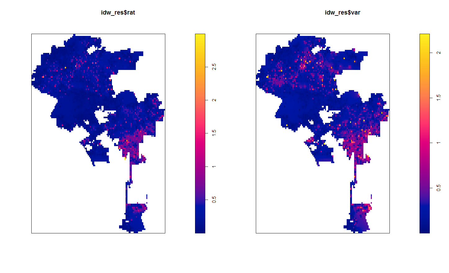

So contrary to expectations, this does not provide a very smooth map. It is quite rough. This is partially because social science data is not going to be as regular as natural science measurements. In spatial stats jargon street to street measures will have a large nugget – a clean street can be right next to a dirty one.

Here the default is using inverse distance squared – what if we just use inverse distance though?

#Inverse distance (linear)
idw_Lin <- idw2(LA_StreetPP, power=1)
plot(idw_Lin$rat)
plot(idw_Lin$var)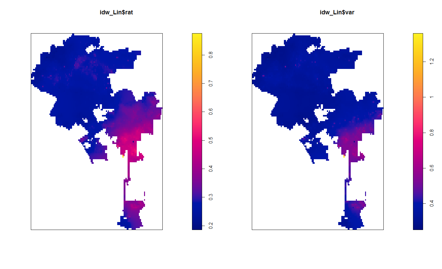

This is smoothed out a little more. There is essentially one dirty spot in the central eastern part of the city (I don’t know anything about LA neighborhoods). Compared to the first set of maps, the dirty streets in the northern mass of the city are basically entirely smoothed out, whereas before you could at least see little spikes.

So I was wondering if there could maybe be better weights we could choose to smooth out the data a little better. One I have used in a few recent projects is the bisquare kernel, which I was introduced by the geographically weighted regression folks. The bisquare kernel weight equals [1 - (d/b)^2]^2, when d < b and zero otherwise. Here d is the distance, and b is a user chosen distance threshold. We can make a plot to illustrate the difference in weight functions, here using a bisquare kernel distance of 2000 meters.

#example weight functions over 3000 meters
dist <- 1:3000
idw1 <- 1/dist
idw2 <- 1/(dist^2)
b <- 2000
bisq <- ifelse(dist < b, ( 1 - (dist/b)^2 )^2, 0)
plot(dist,idw1,type='l')
lines(dist,idw2,col='red')
lines(dist,bisq,col='blue')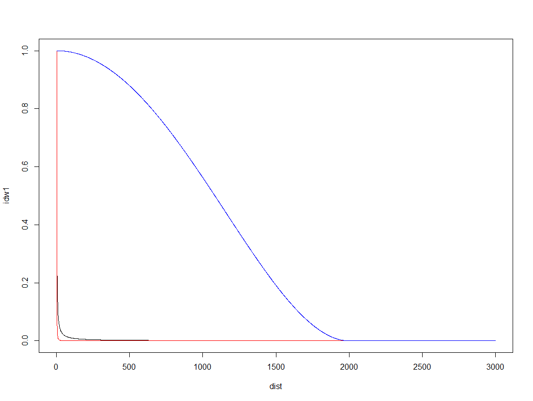

Here you can see both of the inverse distance weighted lines trail to zero almost immediately, whereas the bisquare kernel trails off much more slowly. So lets check out our maps using a bisquare kernel with the distance threshold set to 2000 meters. The biSqW function is equivalent to the original spatstat idw function, but uses the bisquare kernel and returns the variance estimate as well. You just need to pass it a distance threshold for the b_dist parameter.

#BiSquare weighting, 2000 meter distance
LA_bS_w <- biSqW(LA_StreetPP, b_dist=2000)
plot(LA_bS_w$rat)
plot(LA_bS_w$var)

Here we get a map that looks more like a typical hot spot kernel density map. We can see some of the broader trends in the northern part of the city, and even see a really dirty hot spot I did not previously notice in the northeastern peninsula.

The 2,000 meter distance threshold was just ad-hoc though. How large or small should it be? A quick check of the spatial correlogram is one way to make it slightly more objective. Here I use the correlog function in the ncf package to estimate this. I subsample the data first (I presume it has a call to dist somewhere).

#correleogram, random sample, it is too big
subSamp <- CleanStreets[sample(nrow(CleanStreets), 3000), ]
fit <- correlog(x=subSamp$XMidPoint,y=subSamp$YMidPoint,z=subSamp$StreetScor, increment=100, resamp=0, quiet=TRUE)
plot(fit)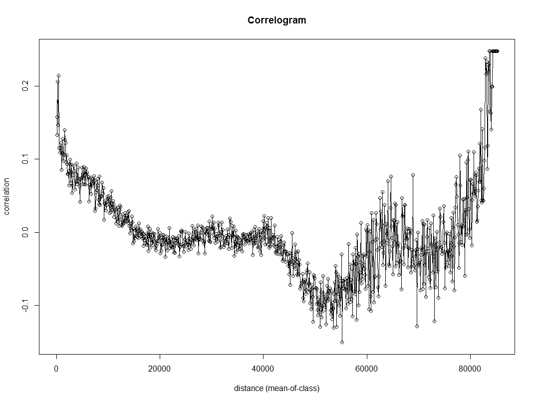

Here we can see points very nearby each other have a correlation of 0.2, and then this trails off into zero before 20 kilometers (the distances here are in meters). FYI the rising back up in correlation for very large distances often occurs for data that have broader spatial trends.

So lets try out a bisquare kernel with a distance threshold of 10 kilometers.

#BiSquare weighting, 10000 meter distance
LA_bS_w <- biSqW(LA_StreetPP, b_dist=10000)
plot(LA_bS_w$rat)
plot(LA_bS_w$var)

That is now a bit oversmoothed. But it allows a nicer range of potential values, as oppossed to simply sticking with the inverse distance weighting.

A few notes on the variance of IDW

So I hacked the idw function in the spatstat package to return the variance of the estimate as well as the actual weighted mean. This involved going into the C function, so I use the inline package to create my own version. Ditto for creating the maps using the bisquare weights instead of inverse distance weighting. To quick see those functions here is the R code.

Given some harassment on Crossvalidated by Mark Stone, I also updated the algorithm to be a more numerically safe one, both for the weighted mean and the weighted variance. Note though that that Wikipedia article has a special definition for the variance. The correct Bessel correction for weighted data though (in this case) is the sum of the weights (V1) minus the sum of square of the weights (V2) divided by V1. Here I just divide by V1, but that could easily be changed (not sure if in the sum of squares I need to worry about underflow). I.e. change the line MAT(var, ix, iy, Ny) = m2 / sumw; to MAT(var, ix, iy, Ny) = m2 / (sumw - sumw/sumw2); in the various C calls.

Someone should also probably write in a check to prevent distances of zero. Maybe by capping the weights to never be above a certain value, although that is not trivial what the default top value should be. (If you have data on the unit square weights above 1 would occur quite regularly, but for a large city like this projected in meters capping the weight at 1 would be fine.)

In general these variance maps did not behave like I expected them to, either with this or other data. When using Bessel’s correction they tended to look even weirder. So I would need to explore some more before I go and recommend them. Probably should not waste more time on this though, and just fit an actual kriging model though to produce the standard error of the estimates.