Here is a general data science snafu I have seen on multiple occasions. You have some categorical variable with a very high cardinality, say 1000 categories. Well, we generally represent categorical values as dummy values. Also for high cardinality data, we often use PCA to reduce the number of dimensions.

So why not one hot encode the data and then use PCA to solve the problem? As the title of the post says, this does not make sense (as I will show in a bit). Here on the data science stackexchange we have this advice, and I have gotten this response at a few data science interviews so far. So figured a blog post why this does not make sense is in order.

I will show an example using python. First here are the libraries we will be using, and some helper functions to work with sklearn’s pca models.

################################################
# Libraries we need and some functions to 
# work with PCA model object

import numpy as np
import pandas as pd
from sklearn.decomposition import PCA

# via https://scentellegher.github.io/machine-learning/2020/01/27/pca-loadings-sklearn.html
def pca_loadings(mod,data):
    load = mod.components_.T
    list_PC = ['PC' + str(i+1) for i in range(load.shape[0])]
    loadings = pd.DataFrame(mod.components_.T, 
                            columns=list_PC, 
                            index=list(data))
    print(loadings.round(3))
    return loadings

# nice print function for variance explained
def var_exp(mod):
    var_rat = mod.explained_variance_ratio_
    list_PC = ['PC' + str(i+1) for i in range(var_rat.shape[0])]
    ve = pd.DataFrame(var_rat,index=list_PC,columns=['VarExplained'])
    print(ve.round(3))
    return ve

# Returns a nicer dataframe after transform with named PC columns
def nice_trans(mod,data):
    np_dat = mod.transform(data)
    list_PC = ['PC' + str(i + 1) for i in range(np_dat.shape[1])]
    pd_dat = pd.DataFrame(np_dat,columns=list_PC,index=data.index)
    return pd_dat

################################################

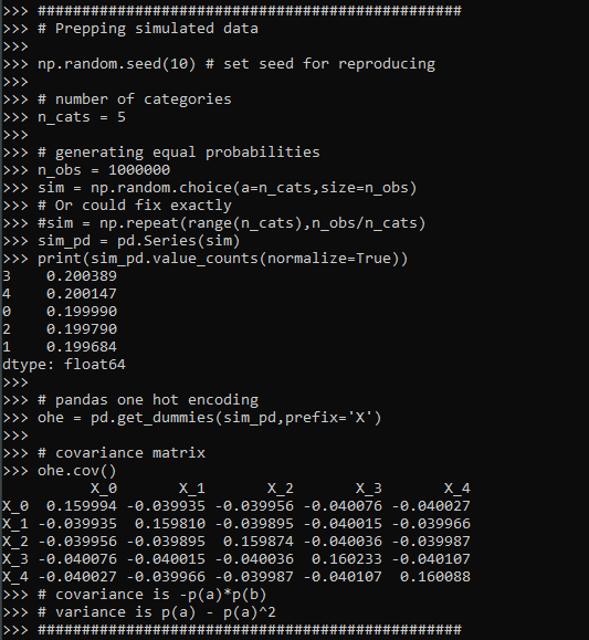
Now lets simulate some simple data, where we have 5 categories, and each category has the same overall proportion in the data. Then we turn that into a one-hot encoded matrix (so 5 dummy variables). We will be using the covariance matrix to do the PCA decomposition (but does not really matter), and the covariance matrix has a nice closed form solution just based on the proportions.

################################################
# Prepping simulated data

np.random.seed(10) # set seed for reproducing

# number of categories
n_cats = 5

# generating equal probabilities
n_obs = 1000000
sim = np.random.choice(a=n_cats,size=n_obs)
# Or could fix exactly
#sim = np.repeat(range(n_cats),n_obs/n_cats)
sim_pd = pd.Series(sim)
print(sim_pd.value_counts(normalize=True))

# pandas one hot encoding
ohe = pd.get_dummies(sim_pd,prefix='X')

# covariance matrix
ohe.cov()
# covariance is -p(a)*p(b)
# variance is p(a) - p(a)^2
################################################

Now we are ready to fit the PCA model on the one hot encoded variables.

# Fitting the PCA and extracting loadings
pca_mod = PCA()
pca_mod.fit(ohe) #based on covariance matrix

# The loadings matrix
bin_load = pca_loadings(pca_mod,ohe)

# showing what the transform looks like on simple data
simple_ohe = pd.DataFrame(np.eye(n_cats,dtype=int),columns=list(ohe))
print( nice_trans(pca_mod,simple_ohe).round(3) )

And we can see all looks ok, minus the final principal component is a constant. This is because when we use all five dummy variables in a one-hot encoded matrix, one column is a linear transformation of the others. So the covariance matrix is just short of being full rank by 1 variable. (Hence why for various algorithms, such as regression, we typically drop one of the dummy variables.)

So typically we interpret PCA as an information compressor – we try to squeeze much of our variance into a smaller number of dimensions. You can interpret each principal component as contributing to the overall variance, and here is that breakdown for our example:

# Showing variance explained
var_equal = var_exp(pca_mod)

So you can see that our reduction in information is not a reduction at all. Typically if we had say 100 dimensions, we may only take the first 10 principal components. While we could do that here, it doesn’t gain us anything. It will essentially be no different than just using the dummy variables for the top k most frequent categories – which with essentially equal categories is just a random set of 10 possible dummy variables.

What about if we do unequal proportions?

#################################################
# What happens with variance explained for unequal 
# proportions?

n_probs = [0.75,0.15,0.05,0.045,0.005]
sim = np.random.choice(a=n_cats,size=n_obs,p=n_probs)
sim_pd = pd.Series(sim)
print(sim_pd.value_counts(normalize=True))
ohe = pd.get_dummies(sim_pd,prefix='X')
print(ohe.cov())

pca_mod_unequal = PCA()
pca_mod_unequal.fit(ohe)

# Showing variance explained
var_unequal = var_exp(pca_mod_unequal)

# Showing the loadings
bin_load_unequal = pca_loadings(pca_mod_unequal,ohe)
#################################################

You can see that the variance explained is similar to the overall proportions in the data. Using the first k principal components will not be exactly the same as keeping the k most frequent categories in the data, as you can see the loading matrix has a particular format (signs can be flipped, PC1 loads opposite on top category and 2nd category, then PC2 loads high on 1,2 and opposite on 3, etc., so looks offhand similar to some type of contrast encoding). But there is no reason offhand to think it will result in a better fit for your particular data than taking the top K (or fitting a model for all dummy variables). (This is generally true for any data reduction via PCA though.)

I attempted to derive a general formula for the eigenvalues from the base proportions, but I was unable to (that determinant and characteristic polynomial form is tricky!). But it appears to me that they mostly just follow the overall proportions in the data. (See at the end of post showing the form of the covariance matrix, and failed attempt at using sympy to derive a general form for the eigenvalues.)

Here is another example with 1000 categories with random probabilities drawn from a uniform distribution. I can generate the eigenvalues without generating a big simulated dataset, since the covariance matrix has a particular form just based on the proportions.

#################################################
# Lets try with a very high cardinality

many_cats = 1000
n_probs = np.random.random(many_cats)
n_probs /= n_probs.sum()
n_probs = -np.sort(-n_probs)
# ?sorted makes the eigenvalues sorted as well?

# I can calculate the eigenvalues without
# generating the big dataset

def ohe_pca(probs):
    # Creating the covariance matrix
    p_len = len(probs)
    pnp = np.array(probs).reshape((p_len,1)) #2d array
    cov = -np.dot(pnp,pnp.T)
    np.fill_diagonal(cov, pnp - pnp**2)
    plabs = ['PC' + str(i+1) for i in range(p_len)]
    cov_pd = pd.DataFrame(cov,columns=plabs,index=plabs)
    # SVD of covariance
    loadings, eigenvals, vh = np.linalg.svd(cov, hermitian=True)
    print('Variance Explained')
    print( (eigenvals / eigenvals.sum()).round(3) )
    return cov_pd, eigenvals, loadings

covbig, eig, load = ohe_pca(n_probs)
#################################################

And here you can see again that the variance explained for each component essentially just follows the overall proportion for each distinct category in the data.

So you don’t gain anything by doing PCA on a one hot encoded matrix, besides creating a more complicated rotation of your binary data.

Covariance of one-hot-encoded and sympy

So first, I state in the comments that the covariance matrix for one-hot encoded variables takes on the form Cov(a,b) = -p(a)p(b). So the definition of the covariance between two values a and b is below, where E[] is the expected value operator.

Cov(a,b) = E[ (a - E[a])*(b - E[b]) ]

For binary variables 0/1, E[a] = p(a), where p(a) is the proportion of 1’s in the column vector. So we can make that replacement above and then expand the inner multiplications:

E[ (a - p(a))*(b - p(b)) ] = 

E[ a*b - a*p(b) - p(a)*b + p(a)*p(b) ]

Due to bilinearity of the expected value, we can then break this down into:

E[a*b] - E[a*p(b)] - E[p(a)*b] + E[p(a)*p(b)]

The value E[a*b] = 0, because the categories are mutually exclusive (if one is 1, the other is 0). The value E[a*p(b)] means multiply the vector of a values by the proportion of b and take the expected value. For a vector of 0’s and 1’s, this reduces to simply p(a)*p(b). So by that logic we have:

0 - p(a)*p(b) - p(a)*p(b) + p(a)*p(b)

-p(a)*p(b)

This same logic works for the variance, except the term E[a*b] is now E[a*a], which does not equal zero, but for a vector of 0’s and 1’s just equals itself, and so reduces to p(a), hence for the variance we have:

p(a) - p(a)^2 = p(a)*(1 - p(a))

I have attempted to write the covariance matrix in this form, and then determine a closed form expression for the eigenvalues, but no luck so far. Here are my attempts to let the sympy python library help. You can see even for a covariance matrix of only three categories, the symbolic representation of the eigenvalues is pretty hairy. So not sure if any simplification is possible:

import sympy

# Returns a covariance matrix
# and proportion dictionary
# in sympy
def covM(n):
    pdict = {}
    for i in range(n):
        pstr = 'p_' + str(i+1)
        pdict[pstr] = sympy.Symbol(pstr,positive=True)
    mlist = []
    for i in range(n):
        a = 'p_' + str(i + 1)
        aex = pdict[a]
        mrow = []
        for j in range(n):
            b = 'p_' + str(j + 1)
            bex = pdict[b]
            if a == b:
                mrow.append(aex*(1 - aex))
            else:
                mrow.append(-aex*bex)
        mlist.append(mrow)
    M = sympy.Matrix(mlist)
    return M, pdict


M, ps = covM(3) #cannot do 5 roots!
ev = M.eigenvals()
ev_list = [k for k in ev.keys()]
e1 = ev_list[0]
print( e1 )

# Not sure how to simplify/collect/whatever
# Into a simpler expression

If you can simplify that I am all ears! (Maybe should be working with M.charpoly() instead?)