Here is a trick I have seen on several occasions people could take advantage of to make fitting models for big data more convenient. If you are using data that is all categorical and a fairly small number of variables, you can aggregate your data and fit models using weights, instead of fitting models on the original micro level data.

For a recent example at my work, was working on a model that originally has around 6 million observations and around a dozen categorical inputs (each with fairly high cardinality, e.g. around 1000 different categories). When aggregating to unique cases, this model is well under half a million rows though. It is much easier for me to iterate and fit models on the half a million row dataset than the 6 million row one.

Here I will show an example using NIBRS data. See my prior blog post on Association Rules for background on the data, I will be using the 2012 NIBRS dataset, which has over 5 million observations. Below is python code to illustrate, but pretty much all statistical packages allow you weight observations.

So first I load the libraries I will be using, and make a nice function to print out the logit coefficients for a sklearn model.

import pandas as pd
import numpy as np
from scipy.stats import binom
from sklearn.linear_model import LogisticRegression
from sklearn.metrics import roc_auc_score

# Function to pretty print logit coefficients
def nice_coef(mod,x_vars):
    coef = list(mod.coef_[0]) + list(mod.intercept_)
    vlist = x_vars + ['Intercept']
    return pd.DataFrame(zip(vlist,coef),columns=['Var','Coef'])

Next we can read in my NIRBS data directly from the dropbox link (replace www with dl to do this in general for dropbox links).

# See https://github.com/apwheele/apwheele.github.io/tree/master/MathPosts/association_rules
# For explanation behind NIBRS data
ndum = pd.read_csv('https://dl.dropbox.com/sh/puws33uebzt9ckd/AADVM86qPJVqP4RHWkWfGBzpa/NIBRS_DummyDat.csv?dl=0')
# If you want to read original NIRBS data
# use https://dl.dropbox.com/sh/puws33uebzt9ckd/AACL3wBhZDr3P_ZbsbUxltERa/NIBRS_2012.csv?dl=0

This data is already prepped with the repeated dummy variables for different categories. It is over 5 million observations, but a simple way to work with this data is to use a groupby and create a weight variable:

group_vars = list(ndum)
ndum['weight'] = 1
ndum_agg = ndum.groupby(group_vars, as_index=False).sum() # sums the weight variable

print(ndum.shape)
print(ndum_agg.shape)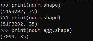

So you can see we went from over 5 million observations to only a few over 7000.

A few notes here. One, if querying the data from a DB, it may be better to do the counts on the DB side and only load in the tinier data into memory, e.g. SELECT COUNT(ID) AS weight, A1,A2... FROM Table GROUP BY A1,A2,.....

Second, I do not have any missing data here, but pandas groupby will by default drop missing rows. So you may want to do something like data.fillna(-1).groupby, or the option to not drop NA values.

Now, lets go onto to fitting a model. Here I am using logit regression, as it is easier to compare the inputs for the weighted/non-weighted model, but you can do this for whatever machine learning model you want. I am predicting the probability an officer is assaulted.

logit_mod = LogisticRegression(penalty='none', solver='newton-cg')
y_var = 'ass_LEO_Assault'
x_vars = group_vars.copy() #[0:7]
x_vars.remove(y_var)

# Takes a few minutes on my machine!
logit_mod.fit(ndum[x_vars],ndum[y_var])

# Coefficients for the model
bigres = nice_coef(logit_mod,x_vars)
bigres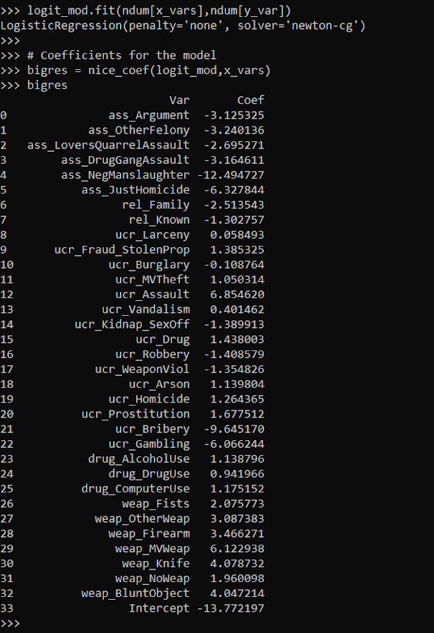

I was not sure if my computer would actually fit this model without running out of memory. But it did crunch it out in a few minutes. Now lets look at the results when we estimate the model with the weighted data. In all the sklearn models you can just pass in a sample_weight into the fit function.

logit_mod.fit(ndum_agg[x_vars],ndum_agg[y_var],sample_weight=ndum_agg['weight'])

weight_res = nice_coef(logit_mod,x_vars)
weight_res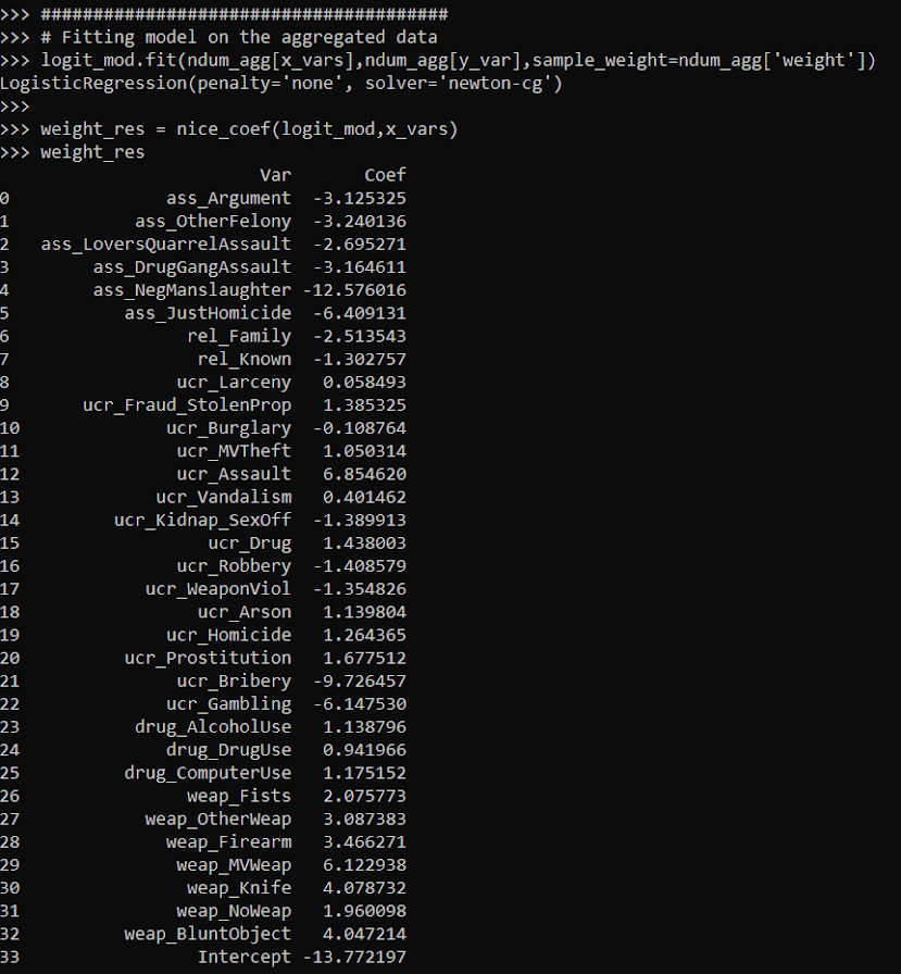

You can see that these are basically the same model predictions. For a few of the coefficients you can find discrepancies starting at the second decimal, but the majority are within floating point errors.

bigres['Coef'] - weight_res['Coef']

This was fit instantly instead of waiting several minutes. For more intense ML models (like random forests), this can dramatically improve the time it takes to fit models.

If you are interested in doing a train/test split, this is quite easy with the weights as well. Basically you just need to allocate some of the weight to the train and some to the test. Here I show how to do that using a binomial random variable. Then you feed the train weights to the fit function:

train_prop = 0.5
train_weight = binom.rvs(ndum_agg['weight'].astype(int), train_prop, random_state=10)
test_weight = ndum_agg['weight'] - train_weight

logit_mod.fit(ndum_agg[x_vars],ndum_agg[y_var],sample_weight=train_weight)

And in sklearn pretty much all of the evaluation functions also take a sample weight function.

pred_probs = logit_mod.predict_proba(ndum_agg[x_vars])

# Eval metrics for the test data
roc_auc_score(ndum_agg[y_var],pred_probs[:,1],sample_weight=test_weight)
roc_auc_score(ndum_agg[y_var],pred_probs[:,1],sample_weight=train_weight)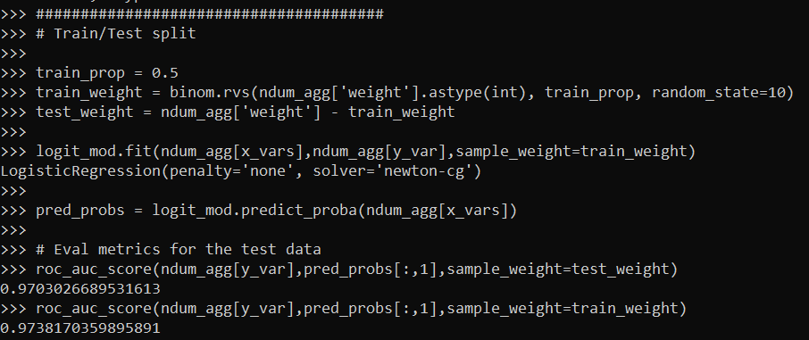

So this shows that the AUC metric decreases in the test dataset (as you would expect it to). Note do not take this model seriously, I would need to think more thoroughly about the selection of rows here, as well as how to effectively interpret these particular categorical inputs in a more reasonable way than eyeballing the coefficients.

I am wondering if weighting the data is actually a more convenient way to do train/test CV splits, just change the weights instead of splitting up datasets. (You could also do fractional weights, e.g. train_weight = ndum_agg['weight']/2, which works nice for stratifying the sample, but may cause some issues generalizing.)

So note this does not always work – but works best with sparse/categorical data. If you have numeric data, you can try to discretize the data to a reasonable amount to still model it as a continuous input (e.g. round age to one decimal, e.g. 20.1). But if you have more than a few numeric inputs you will have a much harder time compressing the data into a smaller number of weighted rows.

It also only works if you have a limited number of inputs. If you have 100 variables you will be able to aggregate less than if you are working with 10.

But despite those limitations, I have come across several different examples in my career where aggregating and weighting the data was clearly the easiest approach, and NIBRS is a great example.