Reference lines for star plots aid interpretation

The other day I was reading Nathan Yau’s Visualize This, and in his chapter on visualizing multi-variate relationships, he brought up star plots (also referred to as radar charts by Wikipedia). Below is an example picture taken from a Michael Friendly conference paper in 1991.


Update: Old link and image does not work. Here is a crappy version of the image, and an updated link to a printed version of the paper.

One of the things that came to mind when I was viewing the graph is that a reference line to signify points along the stars would be nice (similar to an anchor figure I mention in the making tables post on the CV blog). Lo and behold, the author of the recently published EffectStars package for R must have been projecting his thoughts into my mind. Here is an example taken from their vignette on the British Election Panel Study

Although the use case is not exactly what I had in mind (some sort of summary statistics for coefficients in multi-nomial logistic regression models), the idea is still the same. The small multiple radar charts typically lack a scale with which to locate values around the star (see a google image search of star plots to reinforce my assertion) . Although I understand data reduction is necessary when plotting a series of small multiples like this, I find it less than useful to lack the ability to identify the actual value along the star in that particular node. Utilizing reference lines (like the median or mean of the distribution, along with the maximum value) should help with this (at least you can compare whether nodes are above/below said reference line). It would be similar to inserting a guidline for the median value in a parallel coordinates plot (but obviously this is not necessary).

Here I’ve attempted to display what I am talking about in an SPSS chart. Code posted here to replicate this and all of the other graphics in this post. If you open the image in a new tab you can see it in its full grandeur (same with all of the other images in this post).


Lets back up a bit, to explain in greater detail what a star plot is. So to start out, our coordinate system of the plot is in polar coordinates (instead of rectangular). Basically the way I think of it is the X axis in a rectangular coordinate system is replaced by the location around the circumference of a circle, and the Y axis is replaced by the distance from the center of the circle (i.e. the radius). Here is an example, using fake data for time of day events. The chart on the left is a “typical” bar chart, and the chart on the right are the same bars displayed in polar coordinates.

The star plots I displayed before are essentially built from the same stuff, they just have various aesthetic parts of the graph (referred to as “guides” in SPSS’s graphics language) not included in the graph. When one is making only one graphic, one typically has the guides for the reference coordinate system (as in the above charts). In particular here I’m saying the gridlines for the radius axis are really helpful.

Another thing that should be mentioned is, comparing multi-variate data one typically needs to normalize the locations along any node in the chart to make sense. An example might be if one node around the star represents a baseball players batting average, and another represents their number of home runs. You can’t put them on the same scale (which is the radius in a polar coordinate system), as their values are so disparate. All of the home runs would be much closer to the circumferance of the circle, and the batting averages would be all clustered towards the center.

The image below uses the same US average crime rate data from Nathan Yau’s book (available here) to demonstrate this. The frequency that some of the more serious crimes happen, such as homicide, are much smaller than less serious crimes such as assault and burglary. Mapping all of these types of crimes to the same radius in the chart does not make sense. Here I just use points to demonstrate the distributions, and a jittered dot plot is on the right to demonstrate the same problem (but more clearly).

So to make the different categories of crimes comparable one needs to transform the distributions to be on similar scales. What is typically done in parrallel coordinate plots is to rescale the distribution for any variable to between 0 and 1 (a simple example would be new_x = (x – x_min)/(x_max – x_min) where new_x is the new value, x is the old value, x_min is the minimum of all the x values, and x_max is the maximum of all the x values).1 But depending on the data you could use others (if all could be re-expressed as proportions of something would be an example). Here I will rank the data.

1: This re-scaling procedure will not work out well if you have an outlier. There is probably no universal good way to do the rescaling for comparisons like these, and best practices will vary depending on context.

So here the reference guide is not as useful (since the data is rescaled it is not as readily intuitive as the original rates). But, we could still include reference guides for say the maximum value (which would amount to a circle around the star plot) or some other value (like the median of any node) or a value along the rescaled distribution (like the mid-point – which won’t be the same as the original median). If you use something like the median in the original distribution it won’t be a perfect circle around the star.

Here the background reference line in the plot on the left is the middle rank (26 out of 50 states plus D.C.). The background reference line in the plot on the left is the middle rank (26 out of 50 states plus D.C.). The reference guide in the plot on the right is the ranking if the US average were ranked as well (so all the points more towards the center of the circle are below the US average).

Long story short, all I’m suggesting if your in a situation in which the reference guides are best ommitted, an unobstrusive reference guide can help. Below is an example for the 50 states (plus Washington, D.C.), and the circular reference guide marks the 26th rank in the distribution. The plot I posted at the beginning of the blog post is just this sprucced up alittle bit plus a visual legend with annotations.


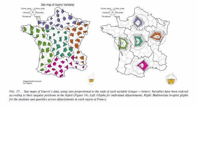
Part of the reason I am interested in such displays is that they are useful in visualizing multi-variate geographic data. The star plots (unlike bar graphs or line graphs) are self contained, and don’t need a common scale (i.e. they don’t need to be placed in a regular fashion on the map to still be interpretable). Examples of this can be found in this map made by Charles Minard utilizing pie charts, Dan Carr’s small glyphs (page 7), or in a paper by Michael Friendly revisiting the moral statistics produced by old school criminologist Andre Guerry. An example from the Friendly paper is presented below (and I had already posted it as an example for visualizng multi-variate data on the GIS stackexchange site).


An example of how it is difficult to visualize lines without a common scale is given in this working paper of Hadley Wickham’s (and Cleveland talks about it and gives an example of bar charts in The Elements). Cleveland’s solution is to provide the bar a container which provides an absolute reference for the length of that particular bar, although it is still really hard to assess spatial patterns that way (the same could probably be said of the star plots too though).

Given models with many spatially varying parameters I think this has potential to be applied in a wider variety of situations. Instances that first come to mind are spatial discrete choice models, but perhaps it could be extended to situations such as geographically weighted regression (see a paper, Visual comparison of Moving Window Kriging Models by Demsar & Harris, 2010 for an example) or models which have spatial interactions (e.g. multi-level models where the hierarchy is some type of spatial unit).

Don’t take this as I’m saying that star charts are a panacea or anything, visualizing geographic patterns is difficult with these as well. Baby steps though, and reference lines are good.

I know the newest version of SPSS has the ability to place some charts, like pie charts, on a map (see this white paper), but I will have to see if it is possible to use polar coordinates like this. Since as US state map is part of the base installation for the new version 20, if it is possible someone could just use this data I presented here fairly easily I would think.

Also as a note, when making these star plots I found this post on the Nabble SPSS forum to be very helpful, especially the examples given by ViAnn Beadle and Mariusz Trejtowicz.


Avoid Dynamite Plots! Visualizing dot plots with super-imposed confidence intervals in SPSS and R

Over at the stats.se site I have come across a few questions demonstrating the power of utilizing dot plots to visualize experimental results.

Also some interesting discussion on what error bars to plot in similar experiments is in this question, Follow up: In a mixed within-between ANOVA plot estimated SEs or actual SEs?

Here I will give two examples utilizing SPSS and R to produce similar plots. I haven’t annotated the code that much, but if you need anything clarified on what the code is doing let me know in the comments. The data is taken from this question on the stats site.


Citations of Interest to the Topic


SPSS Code to generate below dot plot


*******************************************************************************************. data list free /NegVPosA NegVNtA    PosVNegA    PosVNtA NtVNegA NtVPosA.
begin data
0.5 0.5 -0.4    0.8 -0.45   -0.3
0.25    0.7 -0.05   -0.35   0.7 0.75
0.8 0.75    0.65    0.9 -0.15   0
0.8 0.9 -0.95   -0.05   -0.1    -0.05
0.9 1   -0.15   -0.35   0.1 -0.85
0.8 0.8 0.35    0.75    -0.05   -0.2
0.95    0.25    -0.55   -0.3    0.15    0.3
1   1   0.3 0.65    -0.25   0.35
0.65    1   -0.4    0.25    0.3 -0.8
-0.15   0.05    -0.75   -0.15   -0.45   -0.1
0.3 0.6 -0.7    -0.2    -0.5    -0.8
0.85    0.45    0.2 -0.05   -0.45   -0.5
0.35    0.2 -0.6    -0.05   -0.3    -0.35
0.95    0.95    -0.4    0.55    -0.1    0.8
0.75    0.3 -0.05   -0.25   0.45    -0.45
1   0.9 0   0.5 -0.4    0.2
0.9 0.25    -0.25   0.15    -0.65   -0.7
0.7 0.6 -0.15   0.05    0   -0.3
0.8 0.15    -0.4    0.6 -0.05   -0.55
0.2 -0.05   -0.5    0.05    -0.5    0.3
end data.
dataset name dynamite.

*reshaping the data wide to long, to use conditions as factors in the plot.

varstocases
/make condition_score from NegVPosA to NtVPosA
/INDEX = condition (condition_score).

*dot plot, used dodge symmetric instead of jitter.
GGRAPH
  /GRAPHDATASET dataset = dynamite NAME="graphdataset" VARIABLES=condition condition_score MISSING=LISTWISE
    REPORTMISSING=NO
  /GRAPHSPEC SOURCE=INLINE.
BEGIN GPL
  SOURCE: s=userSource(id("graphdataset"))
  DATA: condition=col(source(s), name("condition"), unit.category())
  DATA: condition_score=col(source(s), name("condition_score"))
  GUIDE: axis(dim(1), label("condition"))
  GUIDE: axis(dim(2), label("condition_score"))
  ELEMENT: point.dodge.symmetric(position(condition*condition_score))
END GPL.

*confidence interval plot.

*cant get gpl working (maybe it is because older version) - will capture std error of mean.

dataset declare mean.
OMS /IF LABELS = 'Report'
/DESTINATION FORMAT = SAV OUTFILE = 'mean'.
MEANS TABLES=condition_score BY condition
  /CELLS MEAN SEMEAN.
OMSEND.

dataset activate mean.
compute mean_minus = mean - Std.ErrorofMean.
compute mean_plus = mean + Std.ErrorofMean.
execute.

select if Var1  "Total".
execute.

rename variables (Var1 = condition).

*Example just interval bars.
GGRAPH
  /GRAPHDATASET dataset = mean NAME="graphdataset2" VARIABLES=condition mean_plus
  mean_minus Mean[LEVEL=SCALE]
    MISSING=LISTWISE REPORTMISSING=NO
  /GRAPHSPEC SOURCE=INLINE.
BEGIN GPL
  SOURCE: s2=userSource(id("graphdataset2"))
  DATA: condition=col(source(s2), name("condition"), unit.category())
  DATA: mean_plus=col(source(s2), name("mean_plus"))
  DATA: mean_minus=col(source(s2), name("mean_minus"))
  DATA: Mean=col(source(s2), name("Mean"))
  GUIDE: axis(dim(1), label("Var1"))
  GUIDE: axis(dim(2), label("Mean Estimate and Std. Error of Mean"))
  SCALE: linear(dim(2), include(0))
  ELEMENT: interval(position(region.spread.range(condition*(mean_minus+mean_plus))),
    shape(shape.ibeam))
  ELEMENT: point(position(condition*Mean), shape(shape.square))
END GPL.

*now to put the two datasets together in one chart.
*note you need to put the dynamite source first, otherwise it treats it as a dataset with one observation!
*also needed to do some post-hoc editing to get the legend to look correct, what I did was put an empty text box over top of
*the legend items I did not need.

GGRAPH
  /GRAPHDATASET dataset = mean NAME="graphdataset2" VARIABLES=condition mean_plus
  mean_minus Mean[LEVEL=SCALE]
    MISSING=LISTWISE REPORTMISSING=NO
  /GRAPHDATASET dataset = dynamite NAME="graphdataset" VARIABLES=condition condition_score MISSING=LISTWISE
    REPORTMISSING=NO
  /GRAPHSPEC SOURCE=INLINE.
BEGIN GPL
  SOURCE: s=userSource(id("graphdataset"))
  DATA: condition2=col(source(s), name("condition"), unit.category())
  DATA: condition_score=col(source(s), name("condition_score"))
  SOURCE: s2=userSource(id("graphdataset2"))
  DATA: condition=col(source(s2), name("condition"), unit.category())
  DATA: mean_plus=col(source(s2), name("mean_plus"))
  DATA: mean_minus=col(source(s2), name("mean_minus"))
  DATA: Mean=col(source(s2), name("Mean"))
  GUIDE: axis(dim(1), label("Condition"))
  GUIDE: axis(dim(2), label("Tendency Score"))
  SCALE: linear(dim(2), include(0))
  SCALE: cat(aesthetic(aesthetic.color.interior), map(("Observation", color.grey), ("Mean", color.black), ("S.E. of Mean", color.black)))
  SCALE: cat(aesthetic(aesthetic.color.exterior), map(("Observation", color.grey), ("Mean", color.black), ("S.E. of Mean", color.black)))
  SCALE: cat(aesthetic(aesthetic.shape), map(("Observation", shape.circle), ("Mean", shape.square), ("S.E. of Mean", shape.ibeam)))
  ELEMENT: point.dodge.symmetric(position(condition2*condition_score), shape("Observation"), color.interior("Observation"), color.exterior("Observation"))
  ELEMENT: interval(position(region.spread.range(condition*(mean_minus+mean_plus))),
    shape("S.E. of Mean"), color.interior("S.E. of Mean"), color.exterior("S.E. of Mean"))
  ELEMENT: point(position(condition*Mean), shape("Mean"), color.interior("Mean"), color.exterior("Mean"))
END GPL.
*******************************************************************************************.

R code using ggplot2 to generate dot plot


library(ggplot2)
library(reshape)

#this is where I saved the associated dat file in the post
work <- "F:\\Forum_Post_Stuff\\dynamite_plot"
setwd(work)

#reading the dat file provided in question
score <- read.table(file = "exp2tend.dat",header = TRUE)

#reshaping so different conditions are factors
score_long <- melt(score)

#now making base dot plot
plot <- ggplot(data=score_long)+
layer(geom = 'point', position =position_dodge(width=0.2), mapping = aes(x = variable, y = value)) +
theme_bw()

#now making the error bar plot to superimpose, I'm too lazy to write my own function, stealing from webpage listed below
#very good webpage by the way, helpful tutorials in making ggplot2 graphs
#http://wiki.stdout.org/rcookbook/Graphs/Plotting%20means%20and%20error%20bars%20(ggplot2)/

##################################################################################
## Summarizes data.
## Gives count, mean, standard deviation, standard error of the mean, and confidence interval (default 95%).
##   data: a data frame.
##   measurevar: the name of a column that contains the variable to be summariezed
##   groupvars: a vector containing names of columns that contain grouping variables
##   na.rm: a boolean that indicates whether to ignore NA's
##   conf.interval: the percent range of the confidence interval (default is 95%)
summarySE <- function(data=NULL, measurevar, groupvars=NULL, na.rm=FALSE, conf.interval=.95, .drop=TRUE) {
    require(plyr)

    # New version of length which can handle NA's: if na.rm==T, don't count them
    length2 <- function (x, na.rm=FALSE) {
        if (na.rm) sum(!is.na(x))
        else       length(x)
    }

    # This is does the summary; it's not easy to understand...
    datac <- ddply(data, groupvars, .drop=.drop,
                   .fun= function(xx, col, na.rm) {
                           c( N    = length2(xx[,col], na.rm=na.rm),
                              mean = mean   (xx[,col], na.rm=na.rm),
                              sd   = sd     (xx[,col], na.rm=na.rm)
                              )
                          },
                    measurevar,
                    na.rm
             )

    # Rename the "mean" column
    datac <- rename(datac, c("mean"=measurevar))

    datac$se <- datac$sd / sqrt(datac$N)  # Calculate standard error of the mean

    # Confidence interval multiplier for standard error
    # Calculate t-statistic for confidence interval:
    # e.g., if conf.interval is .95, use .975 (above/below), and use df=N-1
    ciMult <- qt(conf.interval/2 + .5, datac$N-1)
    datac$ci <- datac$se * ciMult

    return(datac)
}
##################################################################################

summary_score <- summarySE(score_long,measurevar="value",groupvars="variable")

ggplot(data = summary_score) +
layer(geom = 'point', mapping = aes(x = variable, y = value)) +
layer(geom = 'errorbar', mapping = aes(x = variable, ymin=value-se,ymax=value+se))

#now I need to merge these two dataframes together and plot them over each other
#merging summary_score to score_long by variable

all <- merge(score_long,summary_score,by="variable")

#adding variables to data frame for mapping aesthetics in legend
all$observation <- "observation"
all$mean <- "mean"
all$se_mean <- "S.E. of mean"

#these define the mapping of categories to aesthetics
cols <- c("S.E. of mean" = "black")
shape <- c("observation" = 1)

plot <- ggplot(data=all) +
layer(geom = 'jitter', position=position_jitter(width=0.2, height = 0), mapping = aes(x = variable, y = value.x, shape = observation)) +
layer(geom = 'point', mapping = aes(x = variable, y = value.y, color = se_mean)) +
layer(geom = 'errorbar', mapping = aes(x = variable, ymin=value.y-se,ymax=value.y+se, color = se_mean)) +
scale_colour_manual(" ",values = cols) +
scale_shape_manual(" ",values = shape) +
ylab("[pVisual - pAuditory]") + xlab("Condition") + theme_bw()
plot
#I just saved this in GUI to png, saving with ggsave wasn't looking as nice

#changing width/height in ggsave seems very strange, maybe has to do with ymax not defined?
#ggsave(file = "Avoid_dynamite.png", width = 3, height = 2.5)
#adjusting size of plot within GUI works just fine

Feel free to let me know of any suggested improvements in the code. The reason I did code both in SPSS and R is that I was unable to generate a suitable legend in SPSS originally. I was able to figure out how to generate a legend in SPSS, but it still requires some post-hoc editing to eliminate the extra aesthetic categories. Although the chart is simple enough maybe a legend isn’t needed anyway.

Another example use of small multiples, many different point elements on a map

I recently had a post at the Cross Validated blog about how small multiple graphs,  AndyW says Small Multiples are the Most Underused Data Visualization. In that post I give an example (taken from Carr and Pickle, 2009) where visualizing multiple lines on one graphs are very difficult. A potential solution to the complexity is to split the line graph into a set of small multiples.

In this example, Carr and Pickle explain that the reason the graphic is difficult to comprehend is that we are not only viewing 6 lines individually, but that when viewing the line graphs we are trying to make a series of comparisons between the lines. This suggests in the graph on the left there are a potential of 30 pairwise comparisons between lines. Whereas, in the small multiple graphics on the left, each panel has only 6 potential pairwise comparisons within each panel.

Another recent example that I came across in my work that small multiples I believe were more effective was plotting multiple points elements on the same map. And the two examples are below.

In the initial map it is very difficult to separate out each individual point pattern from the others, and it is even difficult to tell the prevalence of each point pattern in the map including all elements. The small multiple plots allow you to visualize each individual pattern, and then after evaluating each pattern on their own make comparisons between patterns.

Of course there are some drawbacks to the use of small multiple charts. Making comparisons between panels is surely more difficult to do than making comparisons within panels. But, I think that trade off in the examples I gave here are worth it.

I’m just starting to read the book, How Maps Work, by Alan MacEachren, and in the second chapter he gives a similar example many element point pattern map compared to small multiples. In that chapter he also goes into a much more detailed description of the potential cognitive processes that are at play when we view such graphics (e.g. why the small multiple maps are easier to interpret).  Such as how locations of objects in a Cartesian coordinate system take preference into how we categorize objects (as opposed to say color or shape). Although I highly suggest you read it as opposed to taking my word for it!

References

Carr, Daniel & Linda Pickle. 2009. Visualizing Data Patterns with Micromaps. Boca Rotan, FL. CRC Press.

MacEachren, Alan. 2004. How maps work: Representation, visualization, and design. New York, NY. Guilford Press.

Hacking the default SPSS chart template

In SPSS charts, not every element of the chart is accessible through syntax. For example, the default chart background in all of the versions I have ever used is light grey, and this can not be specified in GPL graphing statements. Many of such elements are specified in chart template files (.sgt extension). Chart template files are just a specific text format organized using an xml tag structure. Below is an example scatterplot with the default chart template for version 19.

You can manually edit graphics and save chart templates, but here I am going to show some example changes I have made in the default chart template. I do this because when you save chart templates by manually editing charts, SPSS has defaults for many different types of charts (one example when it changes are if the axes are categorical or numeric). So it is easier to make widespread changes by editing the main chart template.

The subsequent examples were constructed from a chart template originally from version 17, and I will demonstrate 3 changes I have made to my own chart template.

1) Change the background color from grey to transparent.
2) Make light grey, dashed gridlines the default.
3) Change the font.

Here I just copied and saved my own version of the template renamed in the same folder. You can then open up the files in any text editor. I use Notepad++, and it has a nice default plug-in that allows me to compare the original template file with my updated file. Moving on to how to actually make changes.

1) Change the background color.

The original chart color (in RGB hexidecimal code) is "F0F0F0" (you can open up a default chart to see the decimal representation, 240-240-240). Then I just used this online tool to convert the decimal to hexidecimal, and then you can search the template for this color. The background color is only located in one place in the template file, in a tag nested within an tag. I changed "F0F0F0" to "transparent" as oppossed to another RGB color. One might want to use white for the background as well ("FFFFFF").

2) Make light grey, dashed gridlines the default

Sometimes I can’t figure out how to exactly edit the original template to give me what I want. One way to get the “right” code is to manually apply the edits within the output, and save the chart template file to demonstrate how specific tag elements are structured. To get the gridlines I did this, and figured out that I needed to insert a set of tag with my wanted aesthetic specifications within the tag (that is within a tag). So, in my original chart template file the code was;

and below is what I inserted;

I then inserted the gridlines tag within all of the tags (you have several for different axis’s and whether the axis’s are cateogorical or numeric).

3) Change the font

This one was really easy to change. The default font is Sans-Serif. I just searched the file for Serif, and it is only located within one place, within a tag nested within an tag (near, but not within, the same place as the bacground color). Just change the "SansSerif" text to whatever you prefer, for example "Calibri". I don’t know what fonts are valid (if it is dependent on your system or on what is available in SPSS).

Here is what the same scatterplot at the beginning of the post looks like with my updated chart template.

Besides this my only other advice is combing through the original chart template and using trial and error to change items. For example, for many bar charts the default RGB color is tan (D3CE97). You can change that to whatever you want by just doing a find and replace of that hexidecimal code with another valid hexidecimal color code (like BEBEBE for light grey).

These changes are all arbitrary and are just based on personal preference, but should be enlightening as to how to make such modifications. Other ones I suspect people may be interested in are the default color or other aesthetic schemes (such as point shapes). These are located at the end of my original chart template file within the tags. One for instance could change the default colors to be more printer friendly. It would be easier to save a set of different templates for color schemes (either categorical or continuous) than doing the map statements within GPL all the time (although you would need to have your categories ordered appropriately). Other things you can change are the font sizes, text alignment, plot margins, default pixel size for charts, and probably a bunch of other stuff I don’t know about.

I’ve saved my current chart template file at this Google code site for anyone to peruse (for an updated version see here). I’ve made a few more changes than I’ve listed here, but not many. Let me know in the comments if you have any examples of changing elements in your chart template file!

Below is some quick code that sets the chart templates to the file I made and produces the above scatterplots.


***********************************.
*original template location.
FILE HANDLE orig_temp /name = "C:\Program Files\IBM\SPSS\Statistics\19\template\".
*updated template location.
FILE HANDLE update_temp /name = "E:\BLOG\SPSS\GRAPHS\Hacking_Chart_Template\".
*making fake, data, 100 cases.
input program.
loop #i = 1 to 100.
compute V1 = RV.NORM(0,1).
compute V2 = RV.NORM(0,1).
end case.
end loop.
end file.
end input program.
execute.
*original template.
SET CTemplate='orig_temp\chart_style.sgt'.
*Scatterplot.
GGRAPH
/GRAPHDATASET NAME="graphdataset" VARIABLES=V1 V2 MISSING=LISTWISE REPORTMISSING=NO
/GRAPHSPEC SOURCE=INLINE.
BEGIN GPL
SOURCE: s=userSource(id("graphdataset"))
DATA: V1=col(source(s), name("V1"))
DATA: V2=col(source(s), name("V2"))
GUIDE: axis(dim(1), label("V1"))
GUIDE: axis(dim(2), label("V2"))
ELEMENT: point(position(V1*V2))
END GPL.
*My updated template.
SET CTemplate='update_temp\chart_style(AndyUpdate).sgt'.
*Scatterplot.
GGRAPH
/GRAPHDATASET NAME="graphdataset" VARIABLES=V1 V2 MISSING=LISTWISE REPORTMISSING=NO
/GRAPHSPEC SOURCE=INLINE.
BEGIN GPL
SOURCE: s=userSource(id("graphdataset"))
DATA: V1=col(source(s), name("V1"))
DATA: V2=col(source(s), name("V2"))
GUIDE: axis(dim(1), label("V1"))
GUIDE: axis(dim(2), label("V2"))
ELEMENT: point(position(V1*V2))
END GPL.
***********************************.

Some example corrgrams in SPSS base graphics

I was first introduced to corrgrams in this post by Tal Gallil on the Cross Validated site. Corrgrams are visualization examples developed by Michael Friendly used to visualize large correlation matrices. I have developed a few examples using SPSS base graphics to mimic some of the corrgrams Friendly presents, in particular a heat-map and proportional sized dot plot. I’ve posted the syntax to produce these graphics at the SPSS developer forum in this thread.

Some other extensions could be made in base graphics fairly easily, such as the diagonal hashings in the heat-map, but some others would take more thought (such as plotting different graphics in the lower and upper diagonal, or sorting the elements in the matrix by some other criterion). I think this is a good start though, and I particularly like the ability to super-impose the actual correlations as labels on the chart, like how it is done in this example on Cross Validated. It should satisfy both the graph people and the table people! See this other brief article by Michael Friendly and Ernest Kwan (2011) (which is initially in response to Gelman, 2011) and this post by Stephen Few to see what I am talking about.

One of the limitations of these visualizations is that it simply plots the bi-variate correlation. Friendly has one obvious extension in in the corrgram paper when he plots the bi-variate ellipses and loess smoother line. Other potential readings of interest that go beyond correlations may be examining scagnostic characteristics of distributions (Wilkinson & Wills, 2008) or utilizing other metrics that capture non-linear associations, such as the recent MIC statistic proposed in Reshef et al. (2011). All of these are only applicable to bi-variate associations.

Citations: