I read and very much enjoy Kaiser Fung’s blog Junk Charts. One of the exchanges in the comments to the post, Remaking a great chart, Kaiser asserted it was easier to make the original chart in Excel than in any current programming language. I won’t deny it is easier to use a GUI dialog than learn some code, but here I will present how you would go about making the chart in SPSS’s grammar of graphics. The logic extends part-and-parcel to ggplot2.
The short answer is the data is originally in wide format, and most statistical packages it is only possible (or at least much easier) to make the chart when the data is in long format. This ends up being not a FAQ, but a frequent answer to different questions, so I hope going over such a task will have wider utility for alot of charting tasks.
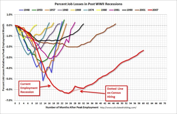
So here is the original chart (originally from the Calculated Risk blog)

And here is Kaiser Fung’s updated version;

Within the article Kaiser states;
One thing you’ll learn quickly from doing this exercise is that this is a task ill-suited for a computer (so-called artificial intelligence)! The human brain together with Excel can do this much faster. I’m not saying you can’t create a custom-made application just for the purpose of creating this chart. That can be done and it would run quickly once it’s done. But I find it surprising how much work it would be to use standard tools like R to do this.
Of course because anyone saavy with a statistical package would call bs (because it is), Kaiser gets some comments by more experienced R users saying so. Then Kaiser retorts in the comments with a question how to go about making the charts in R;
Hadley and Dean: I’m sure you’re better with R than most of us so I’d love to hear more. I have two separate issues with this task:
- assuming I know exactly the chart to build, and have all the right data elements, it is still much easier to use Excel than any coding language. This is true even if I have to update the chart month after month like CR blog has to. I see this as a challenge to those creating graphing software. (PS. Here, I’m thinking about the original CR version – I don’t think that one can easily make small multiples in Excel.)
- I don’t see a straightforward way to proceed in R (or other statistical languages) from grabbing the employment level data from the BLS website, and having the data formatted precisely for the chart I made. Perhaps one of you can give us some pseudo-code to walk through how you might do it. I think it’s easier to think about it than to actually do it.
So here I will show how one would go about making the charts in a statistical package, here SPSS. I actually don’t use the exact data to make the same chart, but there is very similar data at the Fed Bank of Minneapolis website. Here I utilize the table on cumulative decline of Non-Farm employment (seasonally adjusted) months after the NBER defined peak. I re-format the data so it can actually be read into a statistical package, and here is the xls data sheet. Also at that link the zip file contains all the SPSS code needed to reproduce the charts in this blogpost.
So first up, the data from the Fed Bank of Minneapolis website looks like approximately like this (in csv format);
MAP,Y1948,Y1953,Y1957,Y1960,Y1969,Y1973,Y1980,Y1981,Y1990,Y2001,Y2007
0,0,0,0,0,0,0,0,0,0,0,0
1,-0.4,-0.1,-0.4,-0.6,-0.1,0.2,0.1,0.0,-0.2,-0.2,0.0
2,-1.1,-0.3,-0.7,-0.8,0.1,0.3,0.2,-0.1,-0.3,-0.2,-0.1
3,-1.5,-0.6,-1.1,-0.9,0.3,0.4,0.1,-0.2,-0.4,-0.3,-0.1
4,-2.1,-1.2,-1.4,-1.0,0.2,0.5,-0.4,-0.5,-0.5,-0.4,-0.3
This isn’t my forte, so I’m unsure when Kaiser says grab the employment level data from the BLS website what exact data or table he is talking about. Regardless, if the table you grab the data from is in this wide format, it will be easier to make the charts we want if the data is in long format. So in the end if you want the data in long format, instead of every line being a different column, all the lines are in one column, like so;
MAP, YEAR, cdecline
0, 1948, 0
1, 1948, -.04
.
72, 1948, 8.2
0, 2007, 0
1, 2007, 0
.
So in SPSS, the steps would be like this to reshape the data (after reading in the data from my prepped xls file);
GET DATA /TYPE=XLS
 /FILE='data\historical_recessions_recoveries_data_03_08_2013.xls'
   /SHEET=name 'NonFarmEmploy'
   /CELLRANGE=full
   /READNAMES=on
   /ASSUMEDSTRWIDTH=32767.
DATASET NAME NonFarmEmploy.

*Reshape wide to long.
VARSTOCASES
/MAKE cdecline from Y1948 to Y2007
/INDEX year (cdecline).
compute year = REPLACE(year,"Y","").
This produces the data so instead of having seperate years in different variables, you have the cumulative decline in one column in the dataset, and another categorical variable identifying the year. Ok, so now we are ready to make a chart that replicates the original from the calculated risk blog. So here is the necessary code in SPSS to make a well formatted chart. Note the compute statement first makes a variable to flag if the year is 2007, which I then map to the aesthetics of red and larger size, so it comes to the foreground of the chart;
compute flag_2007 = (year = "2007").
GGRAPH
  /GRAPHDATASET NAME="graphdataset" VARIABLES=MAP cdecline flag_2007 year
  /GRAPHSPEC SOURCE=INLINE.
BEGIN GPL
 SOURCE: s=userSource(id("graphdataset"))
 DATA: MAP=col(source(s), name("MAP"))
 DATA: cdecline=col(source(s), name("cdecline"))
 DATA: flag_2007=col(source(s), name("flag_2007"), unit.category())
 DATA: year=col(source(s), name("year"), unit.category())
 SCALE: cat(aesthetic(aesthetic.color), map(("0", color.grey), ("1", color.red)))
 SCALE: cat(aesthetic(aesthetic.size), map(("0",size."1px"), ("1",size."3.5px")))
 SCALE: linear(dim(1), min(0), max(72))
 SCALE: linear(dim(2), min(-8), max(18))
 GUIDE: axis(dim(1), label("Months After Peak"), delta(6))
 GUIDE: axis(dim(2), label("Cum. Decline from NBER Peak"), delta(2))
 GUIDE: form.line(position(*,0), size(size."1px"), shape(shape.dash), color(color.black))
 GUIDE: legend(aesthetic(aesthetic.color.interior), null())
 GUIDE: legend(aesthetic(aesthetic.size), null())
 ELEMENT: line(position(MAP*cdecline), color(flag_2007), size(flag_2007), split(year))
END GPL.
Which produces this chart (ok I cheated alittle, I post-hoc added the labels in by hand in the SPSS editor, as I did not like the automatic label placement and it is easier to add in by hand than fix the automated labels). Also note this will appear slightly different than the default SPSS charts because I use my own personal chart template.

That is one hell of a chart command call though! You can actually produce most of the lines for this call through SPSS’s GUI dialog, and it just takes some more knowledge of the graphic language of SPSS to adjust the aesthetics of the chart. It would take a book to go through exactly how GPL works and the structure of the grammar, but here is an attempt at a more brief run down.
So typically, you would make seperate lines by specifiying that every year gets its own color. This is nearly impossible to distinguish between all of the lines though (as Kaiser originally states). A simple solution is to only highlight the line we are interested in, 2007, and make the rest of the lines the same color. To do this and still have the lines rendered seperately in SPSS’s GPL code, one need to specify the split modifier within the ELEMENT statement (the equivalent in ggplot2 is the group statement within aes). The things I manually edited differently than the original code generated through the GUI are;
- Guide line at the zero value, and then making the guideline 1 point wide, black, and with a dashed pattern (
GUIDE: form.line) - Color and size the 2007 line differently than the rest of the lines (
SCALE: cat(aesthetic(aesthetic.color), map(("0", color.grey), ("1", color.red)))) - Set the upper and lower boundary of the x and y axis (
SCALE: linear(dim(2), min(-8), max(18))) - set the labels for the x and y axis, and set how often tick marks are generated (
GUIDE: axis(dim(2), label("Cum. Decline from NBER Peak"), delta(2))) - set the chart so the legend for the mapped aesthetics are not generated, because I manually label them anyway (
GUIDE: legend(aesthetic(aesthetic.size), null()))
Technically, both in SPSS (and ggplot2) you could produce the chart in the original wide format, but this ends up being more code in the chart call (and grows with the numbers of groups) than simply reshaping the data so the data to makes the lines is in one column.
This chart, IMO, makes the point we want to make easily and succintly. The recession in 2007 has had a much harsher drop off in employment and has lasted much longer than employment figures in any recession since 1948. All of the further small multiples are superflous unless you really want to drill down into the differences between prior years, which are small in magnitude compared to the current recession. Using small lines and semi-transparency is the best way to plot many lines (and I wish people running regressions on panel data sets did it more often!)
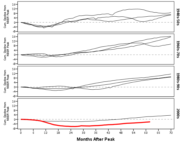
So although that one graph call is complicated, it takes relatively few lines of code to read in the data and make it. In ggplot2 I’m pretty sure would be fewer lines (Hadley’s version of the grammar is much less verbose than SPSS). So, in code golf terms of complexity, we are doing alright. The power in programming though is it is trivial to reuse the code. So to make a paneled version similar to Kaiser’s remake we simply need to make the panel groupings, then copy-paste and slightly update the prior code to make a new chart;
compute #yearn = NUMBER(year,F4.0).
if RANGE(#yearn,1940,1959) = 1 decade = 1.
if RANGE(#yearn,1960,1979) = 1 decade = 2.
if RANGE(#yearn,1980,1999) = 1 decade = 3.
if RANGE(#yearn,2000,2019) = 1 decade = 4.
value labels decade
1 '1940s-50s'
2 '1960s-70s'
3 '1980s-90s'
4 '2000s'.

GGRAPH
  /GRAPHDATASET NAME="graphdataset" VARIABLES=MAP cdecline year decade flag_2007
  /GRAPHSPEC SOURCE=INLINE.
BEGIN GPL
 SOURCE: s=userSource(id("graphdataset"))
 DATA: MAP=col(source(s), name("MAP"))
 DATA: cdecline=col(source(s), name("cdecline"))
 DATA: year=col(source(s), name("year"), unit.category())
 DATA: flag_2007=col(source(s), name("flag_2007"), unit.category())
 DATA: decade=col(source(s), name("decade"), unit.category())
 SCALE: cat(aesthetic(aesthetic.color), map(("0", color.black), ("1", color.red)))
 SCALE: cat(aesthetic(aesthetic.size), map(("0",size."1px"), ("1",size."3.5px")))
 SCALE: linear(dim(1), min(0), max(72))
 SCALE: linear(dim(2), min(-8), max(18))
 GUIDE: axis(dim(1), label("Months After Peak"), delta(6))
 GUIDE: axis(dim(2), label("Cum. Decline from NBER Peak"), delta(2))
 GUIDE: axis(dim(4), opposite())
 GUIDE: form.line(position(*,0), size(size."0.5px"), shape(shape.dash), color(color.lightgrey))
 GUIDE: legend(aesthetic(aesthetic.color), null())
 GUIDE: legend(aesthetic(aesthetic.size), null())
 ELEMENT: line(position(MAP*cdecline*1*decade), color(flag_2007), size(flag_2007), split(year))
END GPL.
It should be easy to see comparing the new paneled chart syntax to the original, it only took two slight changes; 1) I needed to add in the new decade variable and define it in the DATA mapping, 2) I needed to add it to the ELEMENT call to produce paneling by row. Again I cheated alittle, I post hoc edited the grid lines out of the image, and changed the size of the Y axis labels. If I really wanted to automate these things in SPSS, I would need to rely on a custom template. In R in ggplot2, this is not necessary, as everything is exposed in the programming language. This is quite short work. Harder is to add in labels, I don’t bother here, but I would assume to do it nicely (if really needed) I would need to do it manually. I don’t bother here because it isn’t clear to me why I should care about which prior years are which.
On aesthetics, I would note Kaiser’s original panelled chart lacks distinction between the panels, which makes it easy to confuse Y axis values. I much prefer the default behavior of SPSS here. Also the default here does not look as nice in the original in terms of the X to Y axis ratio. This is because the panels make the charts Y axis shrink (but keep the X axis the same). My first chart I suspect looks nicer because it is closer to the Cleveland ideal of average 45 degree banking in the line slopes.
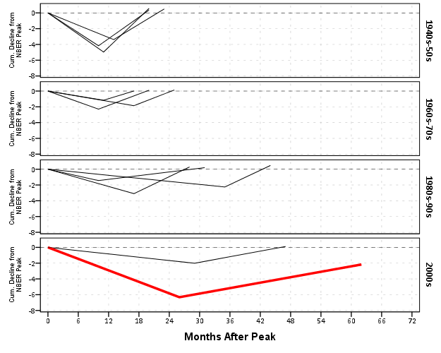
What about the data manipulation Kaiser suggests is difficult to conduct in a statistical programming language? Well, that is more difficult, but certainly not impossible (and certainly not faster in Excel to anyone who knows how to do it!) Here is how I would go about it in SPSS to identify the start, the trough, and the recovery.
*Small multiple chart in piecewise form, figure out start, min and then recovery.
compute flag = 0.
*Start.
if MAP = 0 flag = 1.
*Min.
sort cases by year cdecline.
do if year <> lag(year) or $casenum = 1.
    compute flag = 2.
    compute decline_MAP = MAP.
else if year = lag(year).
    compute decline_MAP = lag(decline_MAP).
end if.
*Recovery.
*I need to know if it is after min to estimate this, some have a recovery before the
min otherwise.
sort cases by year MAP.
if lag(cdecline) < 0 and cdecline >= 0 and MAP > decline_MAP flag = 3.
if year = "2007" and MAP = 62 flag = 3.
exe.
*Now only select these cases.
dataset copy reduced.
dataset activate reduced.
select if flag > 0.
So another 16 lines (that aren’t comments) – what is this world of complex statistical programming coming too! If you want a run-down of how I am using lagged values to identify the places, see my recent post on sequential case processing.
Again, we can just copy and paste the chart syntax to produce the same chart with the reduced data. This time it is the exact same code as prior, so no updating needed.
GGRAPH
  /GRAPHDATASET NAME="graphdataset" VARIABLES=MAP cdecline year decade flag_2007
  /GRAPHSPEC SOURCE=INLINE.
BEGIN GPL
 SOURCE: s=userSource(id("graphdataset"))
 DATA: MAP=col(source(s), name("MAP"))
 DATA: cdecline=col(source(s), name("cdecline"))
 DATA: year=col(source(s), name("year"), unit.category())
 DATA: flag_2007=col(source(s), name("flag_2007"), unit.category())
 DATA: decade=col(source(s), name("decade"), unit.category())
 SCALE: cat(aesthetic(aesthetic.color), map(("0", color.black), ("1", color.red)))
 SCALE: cat(aesthetic(aesthetic.size), map(("0",size."1px"), ("1",size."3.5px")))
 SCALE: linear(dim(1), min(0), max(72))
 SCALE: linear(dim(2), min(-8), max(1))
 GUIDE: axis(dim(1), label("Months After Peak"), delta(6))
 GUIDE: axis(dim(2), label("Cum. Decline from NBER Peak"), delta(2))
 GUIDE: axis(dim(4), opposite())
 GUIDE: form.line(position(*,0), size(size."0.5px"), shape(shape.dash), color(color.lightgrey))
 GUIDE: legend(aesthetic(aesthetic.color.interior), null())
 GUIDE: legend(aesthetic(aesthetic.size), null())
 ELEMENT: line(position(MAP*cdecline*1*decade), color(flag_2007), size(flag_2007), split(year))
END GPL.
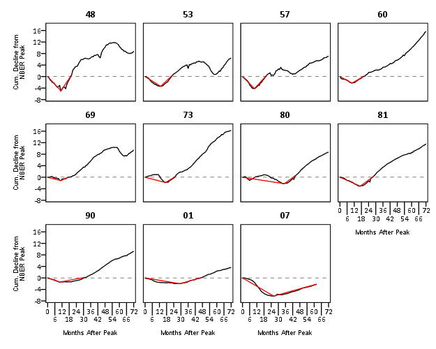
Again I lied a bit earlier, you really only needed 14 lines of code to produce the above chart. I actually spent a few saving to a new dataset. I wanted to see if the reduced summary in this dataset was an accurate representation. You can see it is except for years 73 and 80, in which they had slight positive recoveries before the bottoming out, so one bend in the curve doesn’t really cut it in those instances. Again, the chart only takes some slight editing in the GPL to produce. Here I produce a chart where each year has it’s own panel, and the panels are wrapped (instead of placed in new rows). This is useful when you have many panels.
compute reduced = 1.
dataset activate NonFarmEmploy.
compute reduced = 0.
add files file = *
/file = 'reduced'.
dataset close reduced.
value labels reduced
0 'Full Series'
1 'Kaisers Reduced Series'.

*for some reason, not letting me format labels for small multiples.
value labels year
'1948' "48"
'1953' "53"
'1957' "57"
'1960' "60"
'1969' "69"
'1973' "73"
'1980' "80"
'1981' "81"
'1990' "90"
'2001' "01"
'2007' "07".

GGRAPH
  /GRAPHDATASET NAME="graphdataset" VARIABLES=MAP cdecline year flag_2007 reduced
  /GRAPHSPEC SOURCE=INLINE.
BEGIN GPL
 SOURCE: s=userSource(id("graphdataset"))
 DATA: MAP=col(source(s), name("MAP"))
 DATA: cdecline=col(source(s), name("cdecline"))
 DATA: year=col(source(s), name("year"), unit.category())
 DATA: flag_2007=col(source(s), name("flag_2007"), unit.category())
 DATA: reduced=col(source(s), name("reduced"), unit.category())
 COORD: rect(dim(1,2), wrap())
 SCALE: cat(aesthetic(aesthetic.color), map(("0", color.black), ("1", color.red)))
 SCALE: linear(dim(1), min(0), max(72))
 SCALE: linear(dim(2), min(-8), max(18))
 GUIDE: axis(dim(1), label("Months After Peak"), delta(6))
 GUIDE: axis(dim(2), label("Cum. Decline from NBER Peak"), delta(2))
 GUIDE: axis(dim(3), opposite())
 GUIDE: form.line(position(*,0), size(size."0.5px"), shape(shape.dash), color(color.lightgrey))
 GUIDE: legend(aesthetic(aesthetic.color.interior), null())
 GUIDE: legend(aesthetic(aesthetic.size), null())
 ELEMENT: line(position(MAP*cdecline*year), color(reduced))
END GPL.
SPSS was misbehaving and labelling my years with a comma. To prevent that I made value labels with just the trailing two years. Again I post-hoc edited the size of the Y and X axis labels and manually removed the gridlines. Quite short work. Harder is to add in labels, I don’t bother here, but I would assume to do it nicely (if really needed) I would need to do it manually. I don’t bother here because it isn’t clear to me why I should care
As oppossed to going into a diatribe about the utility of learning a statistical programming language, I will just say that, if you are an analyst that works with data on a regular basis, you are doing yourself a disservice by only sticking to excel. Not only is the tool in large parts limited to the types of graphics and analysis one can conduct, it is very difficult to make tasks routine and reproducible.
Part of my dissapointment is that I highly suspect Kaiser has such programming experience, he just hasn’t taken the time to learn a statistical program thoroughly enough. I wouldn’t care, except that Kaiser is in a position of promoting best practices, and I would consider this to be one of them. I don’t deny that learning such programming languages is not easy, but as an analyst that works with data every day, I can tell you it is certainly worth the effort to learn a statistical programming language well.


jdbutters
/ March 28, 2013My dear chap, you haven’t reproduced the graph. I am with Mr Fung. Once I had the data, it would take me less than five minutes to reproduce that graph in Excel. I doubt I could do it in R — with all the colours and the nice layout — in less than half an hour, and probably it would take much longer to get it perfect. As for updating, I would use FRED’s Excel plug-in and set the spreadsheet up to download the data and update the chart automatically, so I could just open the sheet and press “update data”.
apwheele
/ March 28, 2013Which chart did I not reproduce? I didn’t exactly reproduce the one with 11 colors and gratuitous grid-lines on purpose.
I’m not going to debate how much time it takes in R vs. Excel (that is obviously dependent on your experience in whatever software). The main point was that once you do it one time in a programming language it is done forever. It is not easy to learn how to do it the first time, but to suggest it is easier in Excel because you are ignorant of how to do it another software I find misleading.
Let me know how making a small-multiple chart with facet-wrapped panels goes for you in Excel. There are various other critiques of using Excel for data analysis and data manipulation, so there is no need to go into that.
They are all tools, I want people to make nice charts (and good quantitative decisions) no matter what software you are using. I just made this post to show how you could make such a chart in SPSS.
Yihui
/ March 30, 2013If you want to press “update data”, you are also free to do it in R as well. It is trivial after you have put together the code to fetch the data (e.g. Maciej’s solution below). The source code gives you the ultimate freedom. See RPubs.com for tons of examples on how to generate plots/reports from R.
To clarify, I love GUI in some cases. I do not mean everything should be done by commandline, but the source code is far more transparent and easier to share/reuse/generalize. You can click one button to update one plot for one dataset, and you will have to click a thousand buttons for a thousand datasets — GUI does not scale.
apwheele
/ April 1, 2013Good point – even with just one job my experience is it never ends up being “just a few clicks” – as something or other makes one (annoyingly) repeat the task. I guess that is where the incessant – it must be all done in programming comes from.
Your presence makes me want to write a post on how you can roll it all up into an automated document using SPSS and pandoc – but I doubt anyone will be impressed by my HTML-CSS skills!
Maciej
/ March 29, 2013Here is fast way to download data from this website using R and plot it with ggplot2.
Every plot which is made in Flash has a XML file which contains data. Firebug in Mozilla or Developer Tools in Chrome is very useful to find it out.
In this case direct link to data for emplyment change is below:
http://www.minneapolisfed.org/publications_papers/studies/recession_perspective/parsedxml/employment.xml
To get it directly to R, we can use XML package to parse this file.
library(XML) #to parse xml file
library(reshape2) # to transform data for ggplot2
library(ggplot2)
data<-'http://www.minneapolisfed.org/publications_papers/studies/recession_perspective/parsedxml/employment.xml'
data.xml<-xmlParse(data)
Now we have data in xml, then we shoud transform it to data.frame:
data.df<-xmlToDataFrame(getNodeSet(data.xml,'//series'))
then we add ID for months
data.df$ID<-1:nrow(data.df)
Transform it into data frame for ggplot2
data.long<-melt(data.df,id.vars='ID')
Then, if we want to, change names
names(data.long)<-c('Months','Crisis','Employment')
We should change class of variable Employment (it is character)
class(data.long$Employment)
data.long$Employment<-as.numeric(data.long$Employment)
Now we can plot it with ggplot2.
ggplot(data=data.long,aes(x=Months,y=Employment,colour=Crisis)) + geom_line()
apwheele
/ April 1, 2013Nice example – thank you for sharing!