Lord’s paradox is a situation in which analyzing change scores between two time points results in different treatment effect estimates than analyzing the treatment effect of the second time point conditional on the first time point. In terms of regression equations we have the following as the change score model:

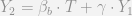
And the following as the conditional model:

Lord’s paradox is the fact that and won’t always be the same. I won’t go into too many details on why that is the case, and I would suggest the reader to review Allison (1990) and Holland and Rubin (1983) for some treatments of the problem. The traditional motivation for the change score model (which is pretty similar to fixed effects in panel regressions) is to account for any time invariant omitted variables that may be correlated with a unit being exposed to the treatment.

So lets say that we have an equation predicting

Lets also say that we cannot observe , we know that it is correlated with , but that does not vary in time. For an example lets say that the treatment is a diet regimen for freshman college students and the outcome of interest is body fat content, and if they sign up they get discounts on specific cafeteria meals. Students voluntarily sign up to take the treatment though, so one may think that certain student characteristics (like being in better shape or have more self control with eating) are correlated with selecting to sign up for the diet. So how can we account for those pre-treatment characteristics that are likely correlated with selection into the treatment?

If we happen to have pre-treatment measures of , we can see that:

And so we can subtract the latter equation from the former to cancel out the omitted variable effect:

Now, a frequent critique of the change score model is that it assumes that the autoregressive effect of the baseline score on the post score is 1. See Frank Harrell’s comment on this answer on the Cross Validated site (also see my answer to that question as to why change scores that include the baseline on the right hand side don’t make sense). Holland and Rubin (1983) make the same assertion. To make it clear, these critiques say that change scores are only justified when in the below equation is equal to 1.

This caused me some angst though. As you can see in my original formulation there is no term at all, so it would seem that if anything I assume it is 0. But it seems that my description of time constant ommitted variables is making the same presumption. To show this lets go back one further step in time:

We can see that we could just replace with the lagged value. Substituting this into the equation predicting we would then have.

Which is the same as saying . So my angst is resolved and Frank Harrell, Don Rubin and Paul Holland are correct in their assertions and doubting such a group of individuals surely makes me crazy! This does bring other questions though as to when the change score model is appropriate. Obviously our models are never entirely correct, and the presumption of is on its face ridiculous in most situations. It is akin to saying the outcome is a random walk that is only guided by various exogenous shocks.

As always, the model one chooses should be balanced against alternatives in an attempt to reduce bias in the effect estimates we are interested in. When the unobserved and omitted is potentially very large and have a strong correlation with being given the treatment, it seems the change score model should be preferred. I presume someone smarter than me can give better quantitative estimates as to when the bias of assuming is a better choice than making the assumption of no other unobserved time invariant omitted variables.

I end this post on a tangent. I recently revisited the material as I wanted to read Holland and Rubin (1983) which is a chapter in the reader Principals of moderns Psychological Measurement: A Festschrift for Frederic M. Lord. I also saw in that same reader a chapter by Melvin Novick, The centrality of Lord’s paradox and exchangeability for all statistical inference. At the end he was pretty daring in making some predictions for the state of statistics as of November 12, 2012 – so I am a year late with my Festschrift but they are still interesting fodder none-the-less. I’ll leave the reader to judge the extent Novick was correct in his following predictions:

1. be less dependent on constricting models such as the normal and will primarily use more general classes of distributions, for example, the exponential power distribution;
2. be fully Bayesian with full emphasis on the psychometric assessment of proper prior distributions;
3. be fully decision theoretic with emphasis on the pyschometric assessment of individual and institutional utilities;
4. use robust classes of prior distributions and utility functions as well as robust model distributions;
5. rely completely on full-rank Bayesian univariate and multivariate analyses of variance and covariance using fully exchangeable, informative prior distributions as appropriate;
6. emphasize exchangeability through careful modeling, blocking, and covariation with randomization playing a residual role;
7. emphasize the use of posterior predictive distributions using the lessons of Lord’s paradox, exchangeability, and appropriate conditional probabilities;
8. place great emphasis on numerical solutions when exact Bayesian solutions prove intractable;
9. still use some pseudo Bayesian methods when both theoretical and computational fully Bayesian solutions remain intractable. (This prevision is subject to modification if I can convince Rubin, Holland and their associates to devote their impressive skills to the quest for fully Bayesian solutions. Should this happen, there may be no need for any pseudo Bayesian methods.)

Citations

• Allison, Paul. 1990. Change scores as dependent variables in regression analysis. Sociological methodology 20: 93-114.
• Holland, Paul & Donald Rubin. 1983. On Lord’s Paradox. In Principles of modern psychological measurement: A festchrift for Frederic M. Lord edited by Wainer, Howard & Samuel Messick pgs:3-25. Lawrence Erlbaum Associates. Hillsdale, NJ.
• Novick, Melvin. 1983. The centrality of Lord’s paradox and exchangeability for all statistical inference. In Principles of modern psychological measurement: A festchrift for Frederic M. Lord edited by Wainer, Howard & Samuel Messick pgs:3-25. Lawrence Erlbaum Associates. Hillsdale, NJ.
• Wainer, Howard & Samuel Messick. 1983. Principles of modern psychological measurement: A festchrift for Frederic M. Lord. Lawrence Erlbaum Associates. Hillsdale, NJ.