
For my advanced research design course this semester I have been providing code snippets in Stata and R. This is the first time I’ve really sat down and programmed extensively in Stata, and this is a followup to produce some of the same plots and model fit statistics for group based trajectory statistics as this post in R. The code and the simulated data I made to reproduce this analysis can be downloaded here.
First, for my own notes my version of Stata is on a server here at UT Dallas. So I cannot simply go
net from http://www.andrew.cmu.edu/user/bjones/traj
net install traj, force
to install the group based trajectory code. First I have this set of code in the header of all my do files now
*let stata know to search for a new location for stata plug ins
adopath + "C:\Users\axw161530\Documents\Stata_PlugIns"
*to install on your own in the lab it would be
net set ado "C:\Users\axw161530\Documents\Stata_PlugIns"
So after running that then I can install the traj command, and Stata will know where to look for it!
Once that is taken care of after setting the working directory, I can simply load in the csv file. Here my first variable was read in as ïid instead of id (I’m thinking because of the encoding in the csv file). So I rename that variable to id.
*Load in csv file
import delimited GroupTraj_Sim.csv
*BOM mark makes the id variable weird
rename ïid id
Second, the traj model expects the data in wide format (which this data set already is), and has counts in count_1, count_2 … count_10. The traj command also wants you to input a time variable though to, which I do not have in this file. So I create a set of t_ variables to mimic the counts, going from 1 to 10.
*Need to generate a set of time variables to pass to traj, just label 1 to 10
forval i = 1/10 {
  generate t_`i' = `i'
}
Now we can estimate our group based models, and we get a pretty nice default plot.
traj, var(count_*) indep(t_*) model(zip) order(2 2 2) iorder(0)
trajplot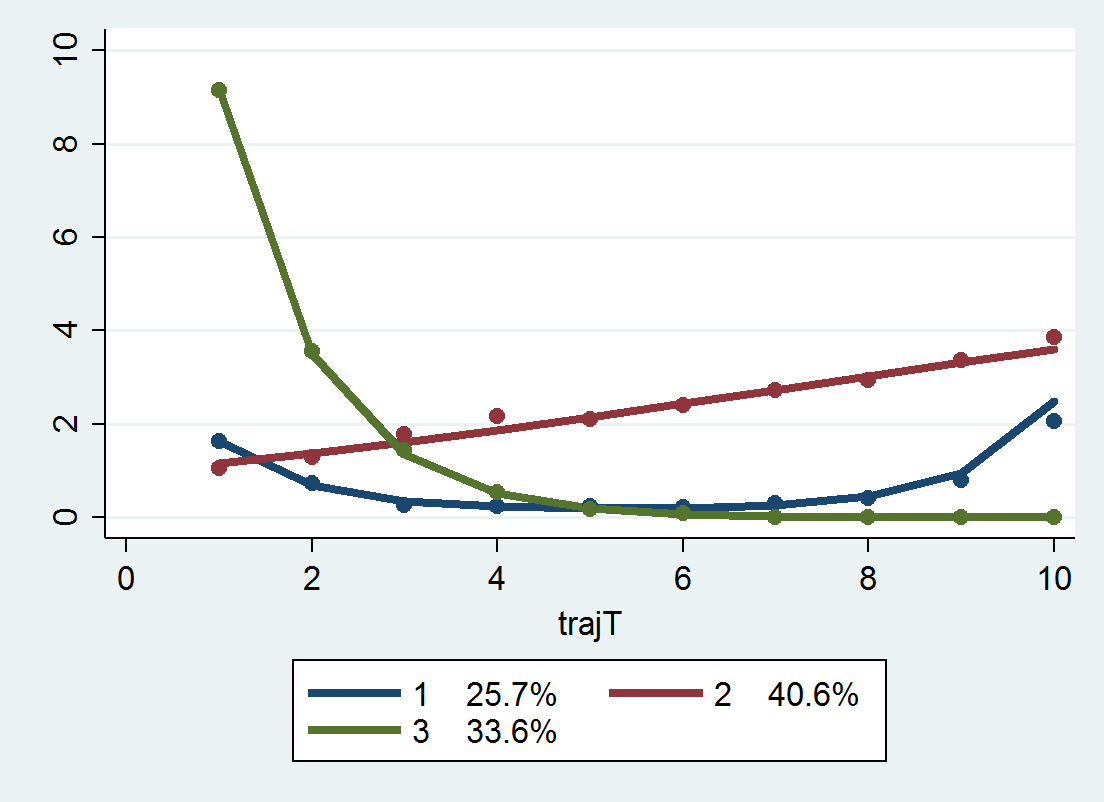
Now for absolute model fit statistics, there are the average posterior probabilities, the odds of correct classification, and the observed classification proportion versus the expected classification proportion. Here I made a program that I will surely be ashamed of later (I should not brutalize the data and do all the calculations in matrix), but it works and produces an ugly table to get us these stats.
*I made a function to print out summary stats
program summary_table_procTraj
    preserve
    *updating code to drop missing assigned observations
    drop if missing(_traj_Group)
    *now lets look at the average posterior probability
	gen Mp = 0
	foreach i of varlist _traj_ProbG* {
	    replace Mp = `i' if `i' > Mp
	}
    sort _traj_Group
    *and the odds of correct classification
    by _traj_Group: gen countG = _N
    by _traj_Group: egen groupAPP = mean(Mp)
    by _traj_Group: gen counter = _n
    gen n = groupAPP/(1 - groupAPP)
    gen p = countG/ _N
    gen d = p/(1-p)
    gen occ = n/d
    *Estimated proportion for each group
    scalar c = 0
    gen TotProb = 0
    foreach i of varlist _traj_ProbG* {
       scalar c = c + 1
       quietly summarize `i'
       replace TotProb = r(sum)/ _N if _traj_Group == c
    }
	gen d_pp = TotProb/(1 - TotProb)
	gen occ_pp = n/d_pp
    *This displays the group number [_traj_~p],
    *the count per group (based on the max post prob), [countG]
    *the average posterior probability for each group, [groupAPP]
    *the odds of correct classification (based on the max post prob group assignment), [occ]
    *the odds of correct classification (based on the weighted post. prob), [occ_pp]
    *and the observed probability of groups versus the probability [p]
    *based on the posterior probabilities [TotProb]
    list _traj_Group countG groupAPP occ occ_pp p TotProb if counter == 1
    restore
end
This should work after any model as long as the naming conventions for the assigned groups are _traj_Group and the posterior probabilities are in the variables _traj_ProbG*. So when you run
summary_table_procTrajYou get this ugly table:
     | _traj_~p   countG   groupAPP        occ     occ_pp       p    TotProb |
     |-----------------------------------------------------------------------|
  1. |        1      103   .9379318   43.57342   43.60432   .2575   .2573645 |
104. |        2      136   .9607258   47.48513   48.30997     .34   .3361462 |
240. |        3      161   .9935605   229.0413   225.2792   .4025   .4064893 |
The groupAPP are the average posterior probabilities – here you can see they are all quite high. occ is the odds of correct classification, and again they are all quite high. Update: Jeff Ward stated that I should be using the weighted posterior proportions for the OCC calculation, not the proportions based on the max. post. probability (that I should be using TotProb in the above table instead of p). So I have updated to include an additional column, occ_pp based on that suggestion. I will leave occ in though just to keep a paper trail of my mistake.
p is the proportion in each group based on the assignments for the maximum posterior probability, and the TotProb are the expected number based on the sums of the posterior probabilities. TotProb should be the same as in the Group Membership part at the bottom of the traj model. They are close (to 5 decimals), but not exactly the same (and I do not know why that is the case).
Next, to generate a plot of the individual trajectories, I want to reshape the data to long format. I use preserve in case I want to go back to wide format later and estimate more models. If you need to look to see how the reshape command works, type help reshape at the Stata prompt. (Ditto for help on all Stata commands.)
preserve
reshape long count_ t_, i(id)
To get the behavior I want in the plot, I use a scatter plot but have them connected via c(L). Then I create small multiples for each trajectory group using the by() option. Before that I slightly jitter the count data, so the lines are not always perfectly overlapped. I make the lines thin and grey — I would also use transparency but Stata graphs do not support this.
gen count_jit = count_ + ( 0.2*runiform()-0.1 )
graph twoway scatter count_jit t_, c(L) by(_traj_Group) msize(tiny) mcolor(gray) lwidth(vthin) lcolor(gray)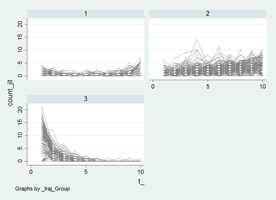
I’m too lazy at the moment to clean up the axis titles and such, but I think this plot of the individual trajectories should always be done. See Breaking Bad: Two Decades of Life-Course Data Analysis in Criminology, Developmental Psychology, and Beyond (Erosheva et al., 2014).
While this fit looks good, this is not the correct number of groups given how I simulated the data. I will give those trying to find the right answer a few hints; none of the groups have a higher polynomial than 2, and there is a constant zero inflation for the entire sample, so iorder(0) will be the correct specification for the zero inflation part. If you take a stab at it let me know, I will fill you in on how I generated the simulation.


mario spiezio
/ April 19, 2018Dear Prof Wheeler, thanks a lot for the code. It is really helpful. I was wondering whether it is possible to use margins after after traj to compute average marginal effects of the covariates included in risk(). Thank you.
apwheele
/ April 19, 2018I don’t think so, it appears you will need to calculate that effect yourself. I’m not sure exactly how you would do it with the mixture model.
Dimi
/ May 7, 2018Dear Prof Wheeler,
Thank you for the code.
For my research, I am trying to use the traj plugin for a survival analysis. As I am not a statistician (I am a physician) you can imagine I need a little help.
My initial issue is that, although I do not have missing values in the long format, in the wide format (due to the fact that some patients died during the follow-up) I do. When I run the code, these patients with “missing values” are dropped from the analysis. Do you know how to overcome this problem?
All my best,
Dimi
apwheele
/ August 13, 2018I am not sure the best way to deal with missing data in such models.
Johan Eriksson
/ November 3, 2022Thanks for the post and all the replies! I have a couple of questions:
1) Is it possible and/or would you recommend to use age as the time-scale? I am struggling to obtain a plot that I‘ve seen in another publication. My dataset has people aged 60 to 100, but if I put their age at each visit in the (indep) option, I get a plot that’s only from 70 to 85, I am guessing that it takes the mean age at each timepoint. What I would like ideally is a plot covering the entire age spectrum, so basically a line smoothing all the individual predicted trajectories in each class.
2) Assuming age doesn’t work out and I go with measurement time, I have five waves where some people are only invited 3 times due to the design of the study. Is it ok for Traj to have missing values in timepoints? So for example one person could have 1 . 1 . 1 for the five time variables, while the other would have 1 1 1 1 1.
3) As I mentioned, I have up to 5 waves of data so I would like to use a quadratic function. Should I exclude those with only 2 observations before running the model, or can they still provide valuable information to the quadratic model?
apwheele
/ November 3, 2022I am not sure about the plot behavior, note you can do something like:
################
traj ….
ereturn list
matrix b = e(b)’
################
To get the coefficients, depending on your equation you can then write a script to feed in different data points (although the superimposed circles on the graph may not make the best sense in that graph).
I imagine you should use age and not measurement time (or I should say there are very few scenarios where I think measure time makes more sense than age).
Like I said in the above comment, I have not checked out the missing data here specifically for the traj command (i.e. I don’t know if it just drops missing data). But, in theory if you have variable input times for your observations, they still contribute. The identification comes from the input points on the curve for everyone, not a single person (you could have only 1 measured point for everyone and still fit a mixture model of age).
Sigrid V
/ December 6, 2022Hi. Thanks for this great resource, and for taking time to reply. I have the same problem as Johan Eriksson, and get the exact same result with cropped age at the x axis (for details, see my entry at Statalist: https://www.statalist.org/forums/forum/general-stata-discussion/general/1691690-disappearing-observations-when-plotting-data-on-a-graph). Have any of you figured this out? I have been struggling for a long time without getting any further. It works fine when I use time of follow-up as time-scale.
Irs
/ November 21, 2023Hi. I have the same problem as you. Have you found the solution?
lori
/ August 12, 2018can you covary outcome group when you have a risk variable?
apwheele
/ August 13, 2018Not exactly sure what you mean — are you asking about a joint trajectory model with multiple outcomes and predicting probability of being in a particular trajectory?
Also to see various examples you can type
help traj
into Stata and it provides various examples.
lori
/ August 13, 2018I have an assessment that is completed across 4 different time points – 12, 18, 24, and 36 months. I am putting scores on a different assessment completed at 6 months as a risk variable. Can I also covary outcome group along with this risk marker to control for diagnosis at 36 months – the outcome group)?
apwheele
/ August 13, 2018I think that would just be something like
traj, var(y1-y4) model(logit) order(2 2 2 2) risk(pre)
if I am understanding correctly. [Sorry if I am not!]
lori
/ August 13, 2018My formulas is traj, var(abc*) indep(time*) model(cnorm) min(53) max(142) order(3) risk(mu6cmss)
When i try to covary for outcome group at the last time point, I get:
. traj, var(abc*) indep(time*) model(cnorm) min(53) max(142) order(3) risk(mu6cmss) cov(dxgroup)
option cov() not allowed
r(198);
. traj, var(abc*) indep(time*) model(cnorm) min(53) max(142) order(3) risk(mu6cmss) tcov(dxgroup)
The number of variables in tcov1 and var1 must match or be a multiple.
r(198);
var has 4 time points, dxgroup has 1 time point
apwheele
/ August 13, 2018tcov is for time-varying covariates. If it is not time varying, it can be used to predict what trajectory group a person in likely to be in, but not the shape of the trajectory over time. Not time-varying covariates should probably go in the “risk()” option in most cases then.
What exactly is “dxgroup”?
lori
/ August 13, 2018dxgroup is the outcome group. We collect data at 12, 18, 24, and 36 months. Then at 36 months, we do a diagnostic check to see if any of our kids end up with a diagnosis of autism. I want to be able to add this into my formula to covariate out any effects of outcome group to check if my predictor variable (an assessment completed at 6 months of age) can predict trajectory membership above and beyond outcome group.
apwheele
/ August 13, 2018Given that description your formula should be:
traj, var(abc*) indep(time*) model(cnorm) min(53) max(142) order(3) risk(mu6cmss dxgroup)
with only one group though this is probably not identified. So you will need to change it to something like:
“order(2 2)” for two trajectory groups or
“order(2 2 2)” for three trajectory groups etc.
(With only four time points I would not do a cubic, about the best you can do is a quadratic).
lori
/ August 13, 2018If you have two risk variables, does it matter what order you put them in, because if i put the 6 month assessment first followed by dxgroup, i get different information.
apwheele
/ August 13, 2018If you mean should
“risk(mu6cmss dxgroup)”
give a different result than
“risk(dxgroup mu6cmss)”
it should not. One caveat is that the labelling of the trajectory groups is arbitrary, so they could in theory converge to the same estimates, but different groups get different labels (and subsequently the coefficients predicting trajectory membership may then be altered).
Given that the mixture models have difficulty converging that could also be a culprit as well.
This is a bit awkward to give so many comments, just send me an email and it will be easier for me to respond.
Yong Kyu Lee
/ August 16, 2018Thank you for the thorough review.
I had a great help from it.
I usually use SAS, so I am not familiar with STATA, but by some political reason I have to do GBTM in STATA.
And I am wondering a way to get a file, as in ‘SAS ods output’, of the result of this GBTM which is ID and designated group by posterior probability.
apwheele
/ August 17, 2018You can just save the results to a csv file. After you run the traj command, something like:
********************
preserve
keep ID _traj*
outsheet using “TrajResults.csv:, replace comma
restore
********************
Risha Gidwani-Marszowski
/ July 18, 2019Thanks so much for this very helpful walkthrough.
I am running the following code with the -traj- program in Stata looking at monthly cost trajectories. Here, t_1-t_12 represent 12 months:
*********************************************************************************************
traj, var(total_cost*) indep(t_*) model(cnorm) min(0) max(748938.3) order (2 2 2)
**********************************************************************************************
I get the following error:
“total_cost2 is not within min1 = 0 and max1 = 748938.3”
The problem is, the maximum value for total_cost2 is actually $748,938.3. So the error doesn’t make sense to me. If I increase the max to 748938.4, I get another error of “unrecognized command.”
Question: How can I avoid getting the top error?
I tried making the “min” and “max” values that exceed the range of the actual cost values in the entire 12-month dataset and that didn’t work.
I tried specifying min(0) and min1…min(12), with the values for min 1…12 being the actual maximum values in the dataset for those months, and got an error for max(7), suggesting I cannot specify past max(6).
apwheele
/ July 22, 2019Sorry for the late approval — vacation last week! I am not sure about that error, the code looks correct to me.
If it is too large of numbers for whatever reason, you can divide by all the dependent variables by a constant (e.g. divide by 10,000). If that does not work I might send Bobby Jones an email with your data and a reproducible example and see if he can give any advice.
A.Carlsen
/ September 11, 2019I have the exact same problem. Did you find a solution to the problem?
Heine Strand
/ August 9, 2019Hi,
I wonder about the BIC and AIC stats in traj and how to decide the number of groups and slopes based on them. We run a model where we follow dementia patients’ cognition over 8 years. A model with two groups with zero slope provided this stats:
0,0: BIC= -3980.05 (N=1554) BIC= -3977.56 (N=449) AIC= -3969.35 ll= -3965.35
While the more reasonable model would be 2 groups with (1,1) or (2,2). For the former, the stats are:
1,1: BIC= -3679.76 (N=1554) BIC= -3676.04 (N=449) AIC= -3663.72 ll= -3657.72
As I understand, lower BIC and AIC values are preferable. Here the 0,0 model has lowest BIC (-3977.56) compared to the 1,1 model (-3676.04), and thereby the model to be preferred? This goes against our expectation of the progression, and the trajplot cleary suggest the 1,1 model to give a better fit. Should we pick the model with smallest absolute BIC/AIC? I see several authors have used this strategy, even if the literature seems to suggest that lowest values are best:
https://stats.stackexchange.com/questions/84076/negative-values-for-aic-in-general-mixed-model.
Can you help us?
apwheele
/ August 9, 2019Yeah it is confusing, most people report AIC/BIC in positive numbers, so a lower value is better fit. Nagin and company always report it the opposite in their software with negative BIC/AIC values, so a higher value (closer to zero) is better.
I’ve never sat down and figured out why different folks do it differently!
So your perceptions match up with your results.
Heine Strand
/ August 9, 2019Thanks, really reassuring! Saved my day 🙂
Hyeonmi
/ September 18, 2019Thanks for your posting. For comparing the results, how can I get a Relative Entropy?
apwheele
/ September 19, 2019I haven’t seen reference to that one in this context — that would be looking at say if you did a mixture of 3 groups vs a mixture of 4 groups? Or are you asking something different?
Viviane
/ September 26, 2019Hi Andrew,
Thanks a lot for your helpful post!
I wonder if the do.file above to generate [groupAPP occ TotProb , etc] can be also applied straightly for logistic models (binary variables) – without any modification.
Many thanks in advance,
Viviane Straatmann
apwheele
/ September 26, 2019It takes advantage of standardized variable names post the traj command. In particular _traj_ProbG* stores the posterior probabilities for each mixture, and _traj_Group stores a integer label for each group.
So if you say you did something like below I think it will work:
****************************
logit y x
predict _traj_ProbG1
gen _traj_ProbG2 = 1 – _traj_ProbG1
gen _traj_Group = (_traj_ProbG1 < 0.5) + 1
summary_table_procTraj
****************************
Where group 1 is the positive class, and group 2 is the 0 class. I haven't given any thought though as to whether this makes sense in this context.
Viviane
/ September 27, 2019Thanks for replying!
I’m using the command below to generate the groups (i’m still working on decisions of trajectory shapes and number of groups):
traj, model(logit) var(poverty_5-poverty_18) indep(year_1-year_5) order(1 1 1)
From this I get the _traj_Group _traj_ProbG1 _traj_ProbG2 _traj_ProbG3, and then I am running your do.file (below), that seems to be working fine.
However, I wanna check with you if the calculation used in your program (tested in your example above with a zip model) also works in a logit model.
program summary_table_procTraj_VSS2
preserve
*now lets look at the average posterior probability
gen Mp = 0
foreach i of varlist _traj_ProbG* {
replace Mp = `i’ if `i’ > Mp
}
sort _traj_Group
*and the odds of correct classification
by _traj_Group: gen countG = _N
by _traj_Group: egen groupAPP = mean(Mp)
by _traj_Group: gen counter = _n
gen n = groupAPP/(1 – groupAPP)
gen p = countG/ _N
gen d = p/(1-p)
gen occ = n/d
*Estimated proportion for each group
scalar c = 0
gen TotProb = 0
foreach i of varlist _traj_ProbG* {
scalar c = c + 1
quietly summarize `i’
replace TotProb = r(sum)/ _N if _traj_Group == c
}
gen d_pp = TotProb/(1 – TotProb)
gen occ_pp = n/d_pp
*This displays the group number [_traj_~p],
*the count per group (based on the max post prob), [countG]
*the average posterior probability for each group, [groupAPP]
*the odds of correct classification (based on the max post prob group assignment), [occ]
*the odds of correct classification (based on the weighted post. prob), [occ_pp]
*and the observed probability of groups versus the probability [p]
*based on the posterior probabilities [TotProb]
list _traj_Group countG groupAPP occ occ_pp p TotProb if counter == 1
restore
end
summary_table_procTraj_VSS2
Thanks again for you support!
Kind regards,
Viviane
apwheele
/ September 27, 2019Sorry I misinterpreted — yes it works the same no matter what the link function for the outcome you are using is. Those stats are all about the latent classes/mixtures, they aren’t tied directly the what the nature of the outcome is.
Viviane
/ September 29, 2019Many thanks, Andrew! 🙂
sylvia
/ November 7, 2019Dear Prof Wheeler,
Thanks for this post. It is very helpful.
I have a question about starting values for maximum likelihood estimation in stata?
Also, how do I estimate entropy?
Thanks.
apwheele
/ November 7, 2019Sorry, won’t be able to help on that end so much. The help has an example of providing starting values. Had another person ask about Entropy — not sure exactly what that means in this context (so if I had an example could likely show how to program it, but need something to go off of).
Priscila
/ November 18, 2019Dear Prof Wheeler. Thank you very much for this post. It was very useful!
I’m working on a 6 points time trajectories with missing data in 5 of them. I’ve heard that traj command can automatically account for the missings but after I ran the analysis (traj command plus your commands for absolute model fit), I realized that something must be wrong. The TotProb is totally different from the p, I´ve also realized that Totprob corresponds exactly to the proportions in the plot (graph), and the p values are identical to those I get from “tab traj_group”. My concern is that that the proportions plotted are totally different from those for traj_group. Do you have any idea why this is happening? Do I have to specify something relating to missings? Thank you very much!
apwheele
/ November 18, 2019That isn’t per se a problem with missing data. “p” is the assignment based on the maximum posterior probability, whereas TotProb is based on the weights assigned for each group. Them not being close suggests a potential problem with absolute fit of the model.
I haven’t personally had a problem with that situation. It may be you have groups that are very similar, so are often near 50% in their group assignment. So in my table if the “GroupAPP” is very low that would also be a sign. So it may mean you need fewer groups I would guess.
Fanz
/ November 26, 2019Hi Prof Wheeler,
I am using the GBTM for the analysis and I’ve found the optimal number of four trajectories, all with a three-order polynomial. I plotted the graph and I am wondering how I could smooth the graph.
Thanks.
apwheele
/ November 26, 2019I don’t understand — the graphs should be pretty smooth already! (Four cubic functions)
Priscila Weber
/ February 18, 2020Hi Professor Wheeler!
I want to use weighted multinomial logistic regression (weights based on posterior probabilities). I know it has been done with latent class analysis which gives you the probabilities at an individual level. Do you know how I can do it with GBTM? I haven’t found the commands in Stata, so I have no idea how to include the weights in the regression! Thank you very much for your attention and shared knowledge
apwheele
/ February 18, 2020Not 100% sure what you mean — you mean you want to predict the probability of belonging to a latent class based on time-invariant characteristics? (Or something else?)
Priscila Weber
/ February 19, 2020Somenthing Else! I already have my trajectories (wheezing trajectories) and also the posterior probabilities of assignment for each group. Now I want to investigate the associations of these trajectories with early risk factors using multinomial logistic regression. However I would like to weight these analyses with the posterior probabilities. It seems that researches are doing this as a way to “account” for uncertainty of assignment. Just to be more “accurate”. It seems that is possible to do it, cause I’ve read it in a paper, but I couldnt find a way to include the weights in the regression! Thank you so much!
apwheele
/ February 22, 2020I am pretty sure you are talking about a model to say why a particular row belongs to a latent group. Check out the “Time-Stable Covariates” section in this document, https://ssrc.indiana.edu/doc/wimdocs/2013-03-29_nagin_trajectory_stata-plugin-info.pdf.
You put in your early risk factors into the “risk(x1 x2 )” part of the function.
Martin CHETEU
/ April 1, 2020Hi professor I am not able to install traj in my Stata 13.here is the message I got when trying to install. I have tried to set the time out but the result is the same. need help plese
net install traj, force
connection timed out — see help r(2) for troubleshooting
could not load traj.pkg from http://www.andrew.cmu.edu/user/bjones/traj/
r(2);
. set timeout1 60
. net install traj, force
connection timed out — see help r(2) for troubleshooting
could not load traj.pkg from http://www.andrew.cmu.edu/user/bjones/tra
apwheele
/ April 1, 2020See if you can download the files yourself first and then install locally. It could just be a server issue at the time you did it.
Safiya Alshibani
/ June 18, 2020Thanks a lot for the example and codes,
I see that some have asked you about the “entropy”. According to the is paper it’s a suggested measure to assess the discrimination between the groups (https://www.ncbi.nlm.nih.gov/pmc/articles/PMC4254619/)
I tried to calculate the entropy for a model with 3 classes as follow (Excuse the primitive way of coding)
gen log_grob1 = ln(_traj_ProbG1)
gen log_grob2 = ln(_traj_ProbG2)
gen log_grob3 = ln(_traj_ProbG3)
gen total_row= (-1*(_traj_ProbG1*log_grob1 + ///
_traj_ProbG2*log_grob2 + ///
_traj_ProbG3*log_grob3)/ln(3))
bys _traj_Group : summ total_row
Q1: do you think my approach of calculating this “entropy” correct ?!
Q2: Also I’m not sure about the threshold, the paper mentioned above suggest a lower value of entropy is better, and other empirical papers suggest higher values are better (i.e. https://journals.sagepub.com/doi/full/10.1177/0081246317721600
https://psycnet.apa.org/record/2010-22993-004
https://link.springer.com/article/10.1007/s00420-017-1277-0)
apwheele
/ June 18, 2020So just reading the pubmed paper, your gen total_row works out as the individual person measure of entropy. For that measure they do not do any group metrics, that one is just for individuals, so the by part doesn’t make sense.
Haven’t read the other papers. Lower values are definitely better, but the pubmed article gives examples where it doesn’t work out so well. (If folks are saying higher values are better, make sure they are calculating the negative in front of the entropy measure, if not then closer to 0 will be better.)
It would take more work to implement the pubmed article suggested hypothesis testing approach. So I won’t be taking that on anytime soon.
Hilary Caldwell
/ July 14, 2020Hi! Thank you for this post, very helpful for getting my trajectories set up. I have two questions:
1) I’m having trouble with the summary stats. I get an error after entering this code:
program summary_table_procTraj
Am I missing something??? Do you enter this after running the model?
2) Do you have experience using an outcome with TRAJ? I’m looking for some help with this.
apwheele
/ July 14, 2020Yeah you should enter it after running the model. It scoops up the variables that the traj model creates to estimate the summary stats.
Not sure what you mean by 2, you mean a time invariant variable predicting the probability of class assignment?
Kate
/ December 2, 2020Hi Prof Wheeler,
Thanks so much for this extremely helpful post and code. I have the same question as others regarding relative entropy. Not sure if this description helps to explain what I mean. It is from the following article: Rens van de Schoot, Marit Sijbrandij, Sonja D. Winter, Sarah Depaoli & Jeroen K. Vermunt (2017) The GRoLTS-Checklist: Guidelines for Reporting on Latent Trajectory Studies, Structural Equation Modeling: A Multidisciplinary Journal, 24:3, 451-467, DOI:10.1080/10705511.2016.1247646
The authors suggest it should be a reporting requirement for trajectory studies.
“The relative entropy is also called a measure of “fuzziness” of the derived latent
classes (Jedidi, Ramaswamy, & DeSarbo, 1993; Ramaswamy, DeSarbo, Reibstein, & Robinson, 1993). The relative entropy takes on a value of 0 when all of the posterior probabilities are equal for each subject (i.e., all participants have posterior probabilities of .33 for each of three latent classes). When each participant perfectly fits in one latent class only, the relative entropy receives a maximum value of 1, which indicates that the latent classes are completely discrete partitions. Therefore, an entropy value that is too low is cause for concern, as it implies that people or cases were not well classified, or assigned to latent classes. Thus, as stated by Celeux and Soromenho (1996) the relative entropy can be regarded as a measure of the ability of the latent trajectory model to provide a relevant partition of the data; a nice explanation is provided by Greenbaum, Del Boca, Darkes, Wang, and Goldman (2005,p. 233).”
Also, a much more basic question: how could I produce a separate trajplot for each group, so the group trajectories are visualised in separate graphs rather than the combined default graph?
Thanks in advance!
apwheele
/ December 2, 2020For the first question, I think this will work (I do not have easy access to Stata anymore to check!). This generates an entropy measure for each individual row in your dataset, not sure how the paper you mention suggests to report this (the mean entropy for the dataset? mean per assigned group?) And you would likely also want to note what the max entropy is, log(n) where n is the number of groups, so you may want to report a normalized entropy value.
##############
gen Ent = 0
foreach i of varlist _traj_ProbG* {
replace Ent = Ent + `i’*log(`i’)
}
replace Ent = -1*Ent
##############
For the question about the graphs, I think this will work:
##############
# check out what is available
preserve
ereturn list
# This gives you the data in the plot
matrix p = e(plot1)
drop _all
svmat p, names(col)
#Plot code here!!!
#This gives you the data in wide format
#So may need to reshape into long
# Now go back to your original data
restore
##############
Siobhan Nowakowski
/ December 23, 2020Hello, I have a very basic question.
I am able to run my GBTM using the code you provided, thank you. However, when I attempt to add risk factors, I get an error message saying “incorrect # of start values. These should be X start vales”. I receive this error message even though I am using the start values provided in the log window.
Are you at all familiar with this issue and how to get around it? Thank you for any help that you can offer
apwheele
/ December 23, 2020Not sure about that one. Is that an error when running my program, or when estimating the GBTM model to begin with? It sounds like the latter.
Siobhan Nowakowski
/ December 23, 2020I use the Proc Traj macro in SAS. I only encounter this problem when adding risk factors after the initial model is estimated. If I run risk factors individually, there is no issue. I may have to do that if I am unable to sort out the problem.
apwheele
/ December 24, 2020I won’t be able to help with that. Maybe emailing the person who created it (Bobby Jones/Dan Nagin) would be your best bet.
Dongling Luo
/ February 22, 2021Hi Prof Wheeler,
Thanks so much for sharing this code. I am wondering whether there’s any restriction for the dependent variables: should the repeated measurements be conformed to normal distribution and do I need to log-transform these data before running GBTM?
Thanks in advance and looking forward to hearing from you soon!
apwheele
/ February 22, 2021The library has examples for different link functions. So normal is one, but you could have 0/1 data, or Poisson count data, and then just use the particular link function that works the best for your data. (So it may make sense to log-transform, or may not if it is say counts of something.)
Dongling Luo
/ February 22, 2021But it seems that the result is different if I log-transform the non-normal distribution data (continuous variable), using the “cnorm” function. I am not sure whether I should log-transform my data (non-normal distribution). Both trajectories seem reasonable. Or could I just simply compare the BIC/AIC to choose the best one? Really appreciate your help!
apwheele
/ February 23, 2021It looks like AIC may be feasible, although you will need to transform the results of the logged model to be comparable to the original scale, https://stats.stackexchange.com/a/343176/1036.
Jane Brathwaite
/ May 18, 2021Hello Prof Wheeler, thank you so much for creating the traj command for Stata. I am wondering, is there any way to know which participants (IDs) are sorted into the respective trajectory groups? I can’t seem to find this info in the output.
apwheele
/ May 18, 2021After you run the command, there should be a variable, _traj_Group, that contains the group that has the highest posterior probability for a person to belong to.
FYI I am not the one who made the traj command itself, I have only blogged about some extra stuff. It was Dan Nagin/Bobby Jones who did the hard work, https://journals.sagepub.com/doi/abs/10.1177/0049124113503141.
Jane Braithwaite
/ May 18, 2021Thank you so much! It worked!
diego yacaman mendez
/ June 28, 2021Hi Andrew,
I noticed you implemented a measure of Entropy in the update of traj for Stata.
How is the entropy calculated? And how should it be interpreted? The lower the better?
Thanks and regards,
apwheele
/ June 28, 2021I am not the person who wrote the original plug in, that is Dan Nagin and Bobby Jones, https://www.andrew.cmu.edu/user/bjones/. So please consult their documentation. But typically higher entropy means things are more random.
Jesús
/ July 28, 2021Hello Prof Wheeler,
Your code was really useful for me. I’m a young PhD student starting modeling trajectories and I’m a bit lost, so I would like to ask you some basic questions. I have three time-points and a continuous variable (it is a metric that goes from 0 to 7).
1. I was using cnorm model. Is it correct or should I use another one?
2. I do not know how to decide the number of groups and the polynomial type for each group trajectory (“order”). How do you decide this? How do you know if you have to put the 0=intercept, 1=linear, 2=quadratic, 3=cubic?
Thanks in advance,
apwheele
/ July 29, 2021For 1 cnorm may make sense/be ok. If it is say a Likert item that only takes on integers from 0-7, some type of ordinal model may be more appropriate.
For 2, with 3 time points the maximum polynomial you can fit is a quadratic. You cannot fit a cubic with only 3 time points.
Nandita Krishnan
/ August 13, 2021Hello, I am using GBTM to estimate dual trajectories of e-cigarette and cigarette use for my dissertation. This is super helpful! In deciding on the final model, one criterion that Nagin recommends is “close correspondence between the estimated probability of group membership and the proportion assigned to that group based on the posterior probability of group membership” – based on the table you generated, would that simply entail comparing p with TotProb?
Also, Nagin recommends “observing reasonably tight confidence intervals around estimated
group membership probabilities”. How are confidence intervals for group membership probabilities calculated? Would it simply be group membership probability (as provided in the stata output after running the model) +/- 1.96 SE?
apwheele
/ August 13, 2021For Q1 yes it is comparing p vs TotProb in these tables.
For Q2 about the CI in membership probabilities I have never seen a calculation of that directly. So maybe a mistake on Nagin’s part? Maybe he mean high posterior probabilities in at least one group? (I have no clue how to estimate individual CI’s, I suppose you could garner that if you have an equation for the membership probabilities, but if you don’t have an equation for that I don’t know.)
Nandita Krishnan
/ August 15, 2021Thank you very much! Another thing I am unsure about is if it is possible to have an APP of 1? I am getting that for a few models and in that case, I am unable to obtain an estimate of occ (as the denominator is 0). Is this theoretically possible or an indication that the model is not viable?
apwheele
/ August 15, 2021It probably does suggest your model is not identified and there is some perfect separation. I have seen this for the trajectory estimates, I have never seen this for the posterior probs though.
Alissa Burnett
/ October 6, 2021I am suddenly having issues with the Traj plug in, Stata 16 and 17 are not recognising the traj command, I get the error message “unrecognized command”
Is anyone else having this issue / have a fix for it?
Nandita Krishnan
/ October 6, 2021I use Stata 14 and I’ve been having issues too – but a different one. where it crashes each time I try to run the traj command. I’ve been able to run it on my university’s virtual computing platform though. Not sure if it’s a Mac issue (do you use a Mac?) or an issue with the traj plug in…
Alissa Burnett
/ October 31, 2021No I’m using a PC and have now tried 3 different computers and it is not working. Reinstalling does not fix the issue.
apwheele
/ October 7, 2021Sorry, won’t get time to check this out for quite a bit. I would just suggest reinstalling and see if that fixes the issue, https://www.andrew.cmu.edu/user/bjones/.
Nandita Krishnan
/ October 27, 2021Does anyone know if it’s possible to model linear splines using the traj plug-in?
apwheele
/ October 27, 2021Since the traj plug-in allows you to incorporate covariates, you could just set the polynomial order term to 0, and include whatever spline basis as covariates in wide format.
Nandita Krishnan
/ October 27, 2021Thank you! Would I use time varying covariates tcov? And if my time variables are coded as t_0 to t_4, and I want the spline at t_1, would I code it as tcov(t_1)?
apwheele
/ October 27, 2021Yes pretty much, (you should likely have the full set of basis functions though, so probably need covariates to t_0, t_1, etc. to make sense). Will try to slate a blog post to illustrate this sometime.
Nandita Krishnan
/ October 27, 2021Will play around with it, thank you! And will keep an eye out for a blog post!
Getu
/ November 25, 2021Hello Prof Wheeler,
Your code was really useful for me. I’m a young PhD student starting modeling trajectories and I’m a bit lost, so I would like to ask you some basic questions. I have thirteen time-points data collected monthly and a continuous variable (height-for-age Z score).
1. I do not know how to decide the number of groups??
2. … And the polynomial type for each group trajectory (“order”). How do you decide this? How do you know if you have to put the 0=intercept, 1=linear, 2=quadratic, 3=cubic?
For example if we have 3 class what is our ground to make the order (1 1 1) or (2 2 2) or (2 3 1) or (3 3 3) etc…
Thanks in advance,
apwheele
/ November 25, 2021In terms of the number of groups, you typically run the models with multiple groups (e.g. 1, 2, 3, etc.) and use the fit AIC/BIC (plus those fit statistics in this post) to identify the best model.
In terms of the polynomial, that should be dictated by your knowledge of the system. Heights are monotonically increasing I presume, and over this short of a time range I believe a linear model will be fine. If you wanted to quadratic as an *approximation* to a non-linear function (although again a function that is only monotonically increasing probably makes more sense). I have a hard time imagining a cubic though with your description.
Getu
/ November 26, 2021Thank you! really helpful.
Jesús martínez Gómez
/ November 26, 2021Hello Getu,
I was in the same point as you several months ago. I highly recommend you the following book: Nagin, D. (2009). Group-based modeling of development. Harvard University Press.
It is really well explained and you would find all your answers. This page website is really helpful too. Thanks Prof Wheeler!
apwheele
/ November 26, 2021Yes agree that book is really good for an introduction — much easier to understand everything than by reading academic papers.
Getu Gizaw
/ November 26, 2021Dear Andrew Wheeler,
Thank you very much! is it freely accessible?
apwheele
/ November 26, 2021Not that I know of — I borrowed it from the Uni library when I was learning this stuff.
Getu Gizaw
/ November 26, 2021oops we from a developing country ( am from Ethiopia) do not have digital care. so kindly request you to attach to me.
Getu
/ December 19, 2021Dear Prof Wheeler,
In follow up of my above question, I am still trying to model Group based trajectory and challenged with -BIC score continues to increase as more groups are added to the model- by using Jeffreys’s scale of evidence for Bayes factors ( using dis exp(BICi−BICj) command.
I also tried Judging Model Adequacy with the following diagnostic criteria:
1. Average Posterior Probability of Assignment
2. Odds of Correct Classification
3. Estimated Group Probabilities versus the Proportion of the Sample Assigned to the Group
4. Confidence Intervals for Group Membership Probabilities
Based on the above four criteria my model is adequate/ accurate starting from having two group and onward.
So, I need your support how to select my best model?
Thank you in advance!
apwheele
/ December 19, 2021Generally you continue to add more groups until they are visibly indistinguishable from each other, or the model itself has difficulty converging.
Getu
/ December 31, 2021Hi prof Apwheele,
Adding more groups still increases BIC ,which makes the model complex and difficulty in model interpretation. i am thinking of convergent problem. so how i can solve this issue in traj model?
thank you!
Sarah B
/ February 23, 2022Thank you for your useful code. Unfortunately when I go to use it in STATA i get the following:
. net from http://www.andrew.cmu.edu/user/bjones/traj
file http://www.andrew.cmu.edu/user/bjones/traj/stata.toc not found
server says file temporarily redirected but did not give new location
http://www.andrew.cmu.edu/user/bjones/traj/ either
1) is not a valid URL, or
2) could not be contacted, or
3) is not a Stata download site (has no stata.toc file).
r(601);
Any ideas what is going wrong?
apwheele
/ February 23, 2022Try https instead of http
Sarah B
/ February 23, 2022Thanks you that’s worked 🙂
Sarah B
/ February 28, 2022Hi,
So I’ve downloaded the traj plug ins but I’m now faced with a “unrecognized command r(199)” error when I try to run my data.
I tried inputting BJones test data and command based on the tutorial found here but I get the same error message.
Click to access lociganic-stata-tutoria.pdf
Any ideas what’s going wrong?
Thanks, Sarah
apwheele
/ February 28, 2022Yeah not sure about that. After install I would do `help traj` like in the linked tutorial. If that pops up I would think the install is OK. If not then the install may not be working out for whatever reason.
Caroline
/ March 31, 2022Hi Andrew,
Nagin mentions in his book that another fit statistic would be the Confidence Intervals for Group Membership Probabilities (so TotProb). Do you know how to add 98% CI’s to the variable?
Thank you for your help and this great article!
Caroline
apwheele
/ March 31, 2022Not 100% sure the correct confidence interval you want. You could maybe do something like:
egen loc_prob =rowmax(_traj_ProbG*)
by _traj_Group: ci means loc_prob, level(98)
Caroline
/ April 5, 2022Thank you!!
It’s the confidence interval or equally I suppose I could use the standard deviation of group membership probabilities (TotProb) for each group. Nagin says that if the intervals are narrow (less than 0.08 plus /minus TotProb) it’s the fourth diagnostic for class enumeration.
Would you still think that the above code gives me what I’m after?
Thanks so much in advance 🙂 it’s really appreciated!
apwheele
/ April 5, 2022Yeah that is the normal based confidence interval given the max posteriori probability for each group. (It may make sense to do a transform since restricted to 0/1, calculate CI on transformed, and then turn the CI back into probabilities, but this is really just a diagnostic, not something being used for actual NHST I believe.)
Since the values are bounded in particular ways, I don’t think this will be very diagnostic above the other stats already presented. Also note the smaller groups can have wider CIs even if the posterior probs have a similar standard deviation.
Raza
/ April 7, 2022Hi Andrew,
I need help in understanding why some trajectories are missing in _traj_Group?
I am using your plugin to run grouped based trajectoy models in Stata. I have 19 years of follow-up and I am using the following syntax and followed is the output of the syntax
traj if group==1, var( exposure_*) indep(t_*) model(zip) order(2 2 2 2 )
Here is an outpt
==== traj stata plugin ==== Jones BL Nagin DS, build: Jan 8 2018
60998 observations read.
51588 excluded by if condition.
9410 observations used in trajectory model.
Maximum Likelihood Estimates
Model: Zero Inflated Poisson (ZIP)
Standard T for H0:
Group Parameter Estimate Error Parameter=0 Prob > |T|
1 Intercept -0.10053 0.02925 -3.437 0.0006
Linear 0.05324 0.00808 6.585 0.0000
Quadratic 0.00140 0.00041 3.404 0.0007
2 Intercept 0.04437 0.02330 1.904 0.0569
Linear 0.00554 0.00573 0.966 0.3341
Quadratic -0.00010 0.00029 -0.343 0.7316
3 Intercept 0.04439 0.00954 4.654 0.0000
Linear 0.00553 0.00228 2.430 0.0151
Quadratic -0.00010 0.00011 -0.878 0.3799
4 Intercept -0.00685 0.02381 -0.288 0.7735
Linear 0.20418 0.00532 38.369 0.0000
Quadratic -0.00746 0.00028 -26.968 0.0000
Group membership
1 (%) 8.65836 0.44359 19.519 0.0000
2 (%) 12.49223 383.21558 0.033 0.9740
3 (%) 69.66792 383.21579 0.182 0.8557
4 (%) 9.18149 0.39125 23.467 0.0000
BIC=-178850.40 (N=155079) BIC=-178829.39 (N=9410) AIC=-178775.77 L=-178760.77
When I tab _traj_Group, it does not return values for trajectory group 2
_traj_Group | Freq. Percent Cum.
————+———————————–
1 | 708 7.52 7.52
3 | 7,855 83.48 91.00
4 | 847 9.00 100.00
————+———————————–
Total | 9,410 100.00
Can you tell what can possibly be wrong here?
apwheele
/ April 7, 2022Well, for my code above it will not be quite right with the missing data, so you could do something like:
program summary_table_procTraj2
preserve
drop if missing(_traj_Group)
….
To fix my code above for your situation.
My guess is that trajectory 2 in your example has no high posterior probabilities, so that variable assigns none of the values to that group. Eyeballing the coefficients, it is very similar to traj group 3. This just suggests you don’t need 4 groups, and 3 will suffice.
My code table above will still not generate summaries for group2 in your scenario. I would have to do some more work, as it relies on the _traj_Group variable.
Raza
/ April 7, 2022That’s correct!
Your response has helped me to understand why STATA is returning missing values.
Thanks a lot!
Lukas
/ May 4, 2022Hi Professor Wheeler,
Thanks for the excellent post! I have a question and would be grateful if you could have a look when you get a chance.
Here is my output:
4300 observations read.
308 had no trajectory data.
3992 observations used in the trajectory model.
But the _traj_Group variable has 4300 nonmissing values (shouldn’t this be 3992?).
How can I determine the 308 observations, and I found there were less than 308 participants who only had 0 or 1 visit. Also, should I say the trajectory is modeled based on 3992 participants or all of the 4300 participants?
Regards,
Lukas
apwheele
/ May 4, 2022If an observation is not used in the trajectory modelling process, I believe it is not assigned posterior probabilities. So maybe filtering the set post that will illustrate what the issues are. I am not sure offhand why it would be dropping cases.
Lukas
/ May 4, 2022Thanks Professor Wheeler. Absolutely, it is very strange that all observations, including those not used in the model, were assigned posterior probabilities. As your suggested, I have double-checked the probabilities of these unused observations and found they have the same posterior probabilities (and very low). Although I’m not sure why this happens, the low posterior probabilities may be a good indicator to identify which observations were not used.
Regards,
Lukas
JM
/ June 2, 2022Professor may I ask if there is a solution for me because I cannot even install the package. Please help me on it.
apwheele
/ June 3, 2022See my note at the beginning of this post, https://andrewpwheeler.com/2021/11/29/splines-in-stata-traj-models/. Try using https, or downloading the data yourself and pointing your Stata install to the local files.
Frederic Theriault
/ August 23, 2022Hello Professor Wheeler,
Thank you for this useful code. It was really helpful. It works great with GBTM in Stata. However, when I’m conducting the code for dual trajectories, and then, put your code afterwards, it gives me just the output for the first trajectory of my dual scripts and not for the other trajectory. Is there any way to specify in the coding that I want outputs for my two trajectories and not juste the first one?
For example, it is my script at the moment:
traj, model(cnorm) var(CD*) indep(Age*) max(12) order(1 1 1 1) var2(bulle*) indep2(Age*) max2(6) model2(cnorm) order2(1 1 1 1 2)
summary_table_procTraj_Toxictrio
Thank you so much!
Frederic Theriault
apwheele
/ August 23, 2022That is not too hard, see https://www.dropbox.com/s/e1dnts3h30964xe/mod2Traj.do?dl=0
Just need to replace “_traj_” in the code with “_traj_Model2_” and everything works the same. Not as familiar with the dual trajectories, so not sure about the stats people use for comparing both.
Frederic Theriault
/ August 23, 2022Wow, this was really helpful, it works perfectly fine! Thank you so much.
Also, I’ve heard that when conducting separately multinomial logistic regression with those trajectories, I shouldn’t do regressions based on class membership (which are automatically given in your data sets once you perform GBTM). It would be more appropriate to perform regressions that are weighted by an individual’s posterior probability of being in a given class. I was then wondering if you know if there is a way to achieve it with those posterior probabilities in the coding here?
Thank you!
Frederic Theriault
apwheele
/ August 23, 2022I am not sure what you mean, can you give a more explicit example regression equation?
Frederic Theriault
/ August 23, 2022For example, to perform a multinomial regression, this is my script (predicting trajectories group membership from theory of mind, with the first group as the reference group) :
mlogit _traj_Group tomtote5, base(1)
_traj_Group is the variable you get automatically in your dataset once you perform GBTM. Its the class membership of each individuals. But there is a risk of uncertainty of assignment, so its more appropriate to take posterior probabilities of each individual for the regression. However, you dont get it automatically in your dataset..
Thank you!
Frederic Theriault
apwheele
/ August 23, 2022Why not just use those as time stable risk factors in the original model, e.g. something like:
traj, model(cnorm) var(CD*) indep(Age*) max(12) order(1 1 1 1) risk(tomtote5) …
Frederic Theriault
/ August 23, 2022Good point! I thought about it but this procedure drops observations with missing risk factor data, so then you don’t have the same trajectories once you add “risk(..). in the script. So in this case, it’s better to conduct regressions separately.
Frederic Theriault
/ August 24, 2022Hi Professor,
the _traj_Group gives for each individual their class membership. Do you know if there is any way on Stata to extract information about each individual posterior probability of being in a given class instead? Is there a command that allows that ? Thank you again!
Frederic
apwheele
/ August 24, 2022It is contained in the “_traj_Prob*” fields, so if you have 3 groups, you will have 3 columns post traj that are _traj_Prob1, _traj_Prob2, _traj_Prob3, etc. Those are the posterior probabilities for belonging to that group.
Frederic Theriault
/ August 25, 2022Oh great thank you so much!
And the tcov option is for time-varying covariate, so it cannot be use with categorical variables such as SES and sex to predict trajectories?
apwheele
/ August 25, 2022Yes — so in the traj model, you have something like:
Outcome^k_t ~ f(t,other_time_varying) # The trajectory equation for group k
Prob(K) ~ f(time_static)
So you have two equations — one estimating the ultimate outcome on the first line (the trajectory), and one estimating the probability of belonging to a particular group (the second line).
If you have constant characteristic, it will not impact the shape of the trajectory over time. It would be confounded with the intercept term in the trajectory equation, since it is a constant over time.
But, it could impact what group you are assigned to (e.g. males more likely to be in one group vs females). Time static covariates are specified via the “risk(…)” option, which is like a multinomial model that predicts the probability of group assignment.
Nandita Krishnan
/ October 24, 2022For a logit model, is there a way to obtain the probabilities of the outcome for each trajectory at each time point? (in other words, is there a way to get the value labels for each of the points plotted in the graph?)
apwheele
/ October 24, 2022Going off of some notes, try something like:
######
traj ….
ereturn list
matrix b = e(b)’
matrix p = e(plot1)
######
To get all the stuff you would need to back out the predictions directly. The p matrix above may be all you need.
Nandita Krishnan
/ October 25, 2022Thank you! This worked perfectly. The p matrix was sufficient.
Luka Van Asche
/ November 6, 2022Hello. I have a cohort followed up two times after baseline, so maximum 3 observations per person. Some people died and dropped out during follow-up. I would like to model the trajectories quadratically, which technically requires at least three time-points. Would I have to exclude everybody who did not come at all 3 occasions before running traj, or could I leave those with two time-points and the model would somehow use their two time-points when calculating the quadratic trajectories?
apwheele
/ November 6, 2022Check out the comments to Johan Eriksson, https://andrewpwheeler.com/2016/10/06/group-based-trajectory-models-in-stata-some-graphs-and-fit-statistics/#comment-18931
Are relevant to this question.
Cori
/ December 3, 2022Hello, thank you for your helpful post! I have a couple of questions:
I tried to run traj model, as below:
traj, var(me_total_*) indep(wave_*) model(zip) order(2 2 2).
It worked when I specified that the number of groups are 3 or less. However, when I tried to increase the number of groups to 4 or more, I got empty outputs with the following message:
“Unable to calculate standard errors. Check model.”
It showed the BIC, AIC, and entropy, but the group parameter estimates, standard error, and group membership were all empty.
Any idea what causes this? Is this considered a converging problem?
My second question, regardless of the number or groups, the output always showed the below message at the bottom of the models:
“warning: variance matrix is nonsymmetric or highly singular.”
What does it mean?
Thank you very much, I would be grateful if you could shed some light.
apwheele
/ December 4, 2022So the variance-covariance warning can be because either the mixture model has some essentially empty groups (so cannot estimate the regression parameter estimates), or it can be because the group for some reason cannot be estimated (say that particular group had no 0’s, so the zero equation cannot be estimated). It is difficult to give more advice just based on the info given in the comment.
Fjorida
/ January 9, 2023Hi Andrew,
Thank you so much for all the codes and replies!
I have a couple of questions and it would be great if you can answer them.
1. For cnorm model do we need normal distributed outcome?
2. What code/model can I use for an ordinal outcome? My outcome has 3 categories (1/2/3).
3. How can I plot in Stata the individual values and means of the outcome by trajectory groups? I tried your codes: gen count_jit = count_ + ( 0.2*runiform()-0.1 )
graph twoway scatter count_jit t_, c(L) by(_traj_Group) msize(tiny) mcolor(gray) lwidth(vthin) lcolor(gray), but I get empty graphs.
4. How can I plot in Stata the individual categories at each time-point by trajectory groups in case of the 3-categorical outcome?
5. Do you in general recommend “age” as time scale? In my project I want to model the longitudinal consumption of alcohol by using 2/3 repeated assessment.
Looking so much forward to your reply.
Thank you!
apwheele
/ January 10, 20231 – No, it can make sense to look at means even if the distribution is clearly non-normal (Likert data is common for example and often reasonable).
2 – Normal may be OK, you may look into other other mixture models with ordinal logit outcomes though, check out the R library flexmix, https://andrewpwheeler.com/2022/04/19/state-dependence-and-trajectory-models/
3 – Not much advice I can give here, note this is after the reshape to long command
4 – I am not sure what you mean here, it may be easier to post to the Stata Forum though to get a quicker answer (have a reproducible example)
5 – Age probably makes the most sense (as opposed to measure time) — just a guess based on simple description. If you are interested in period effects different models may be appropriate (such as age/period/cohort models).
Rjm521
/ March 8, 2023Hello Professor Wheeler,
Thank you for your helpful post. I’ve conducted a trajectory analysis of depression over time amongst a cohort of older adults. I included the dropout extension to account for MNAR, but am having trouble interpreting the provided output:
Maximum Likelihood Estimates
Model: Censored Normal (cnorm)
Standard T for H0:
Group Parameter Estimate Error Parameter=0 Prob > |T|
1 Intercept 41.93368 0.61233 68.482 0.0000
Linear -0.16177 0.08963 -1.805 0.0712
Quadratic 0.00632 0.00318 1.987 0.0470
2 Intercept 54.26351 0.80935 67.045 0.0000
Linear -0.47340 0.10781 -4.391 0.0000
Quadratic 0.01323 0.00378 3.502 0.0005
3 Intercept 64.05830 1.31006 48.897 0.0000
Linear -0.45652 0.22445 -2.034 0.0420
Quadratic 0.01354 0.00862 1.571 0.1162
1 Drop0 -1.31002 0.72209 -1.814 0.0698
Drop1 -0.00415 0.01800 -0.231 0.8177
2 Drop0 -1.10606 1.02995 -1.074 0.2830
Drop1 -0.00753 0.02042 -0.369 0.7124
3 Drop0 0.97593 1.88147 0.519 0.6040
Drop1 -0.02991 0.02979 -1.004 0.3154
Could you help me understand what the estimates for Drop0 and Drop1 are telling me for each group?
Thank you!
apwheele
/ March 8, 2023So for each of groups, you have a second equation that estimates the probability of drop-out conditional on time. Drop0 is the intercept, and Drop1 is the linear trend.
For all three of your groups dropout probability decreases over time by a tiny amount (all have standard errors larger than the coefficient, so can just say time trends are basically 0). Groups 1/2 had negative coefficients for the intercepts so have lower probabilities of dropping out. Group 3 has a positive intercept.
So if you do:
trajplot, dropout
I am guessing it will mostly be 3 straight lines, with Group 1 being around 0.21, Group 2 around 0.25, and Group 3 around 0.73.
Jo
/ June 26, 2023Hi!
Thank you so much for your explanation but I have a really basic question… I dont understand how am I supossed to know the number of groups and the order of polynomial type for each group trajectory… I want to use GBTM precisely because I want to know how many groups are and how they behave, but if I use the command: traj, traj, var() indep() model(zip) order() I need to specify the number of groups and polynomial type in “order”…Is there a previous step to identify number of groups?
Thanks for your help
apwheele
/ June 27, 2023So the number of latent groups is typically not known by the researcher up front, so it is common to use relative metrics to determine the number of groups (e.g. AIC/BIC), or absolute metrics, such as I show here in the table.
Now for the polynomial trends, that tends to have more limits based on understanding of the data (if fewer time periods, you can’t identify higher polynomials, if slowly changing linear may be appropriate). I would suggest using flexible enough terms to capture trends in your data (which may not only be polynomials, but could be other things like splines/breakpoints).
Jo
/ June 27, 2023Oh I understand, but how can I do that in stata? Because everywhere I see they use this command: “traj, var() indep() model(zip) order()” where they already know the number of groups, so thats really my question…
Thank you so much!
apwheele
/ June 27, 2023Not sure I understand the confusion, `var()` is fixed based on your available data in wide format, so there is not really any discretion there. Ditto for `indep()`, see the spline post for an example, https://andrewpwheeler.com/2021/11/29/splines-in-stata-traj-models/.
`model()` doesn’t really have much discretion either, if your data are 0/1 you can’t do a zip model, as zip only makes sense for count data.
For order, again people just look over different orders and look at various stats to choose which model, eg compare
`order(2)` vs `order(2 2)` vs `order(2 2 2)` etc. Eventually it fails to converge, or you get a local min/max in your stats, or you start to get trivial differences in the latent trajectories.
Jo
/ July 2, 2023Thank you so much, I get now!
Fatma
/ July 6, 2023Hi Andrew. I just started running a zip model, and found you syntax to be really helpful. I was wonderning what “iorder(0 -1 0)” really means and changes in the number made within brackets e.g. “iorder(0)” vs ” iorder (1)”.
apwheele
/ July 6, 2023So for zip models there are two equations, the zero-inflated part and the Poisson part. These can have different number of latent categories. So the `iorder` is the same logic as the `order` part, the order part in the zip model is for the Poisson part of the equation.
Fatma
/ July 8, 2023Thank you
Fatma
/ July 21, 2023I have run a series of unconditional models. I would like to progress to conditional models. My first question is what is the minimum acceptable cut-off value for entropy and classification probabilities? Secondly, I have a model with high entropy (>0.9) and high classification probabilities (>0.9). However, the linear, quadratic and intercept estimates are not significant for one class. So, my question is, if fit indices are good, does significance count when selecting a model?
apwheele
/ July 22, 2023There really isn’t a bright line in terms of the absolute fit metrics, Nagin IIRC suggest classification probabilities above 0.7. You could always have a good solution though, and some set of observations are hard to classify into two mixtures.
Probably shouldn’t worry about stat. significance of the coefficients. No intercept/linear/quadratic just means a flat line of 0’s, which may be a totally valid mixture component. Having those extra terms does not bias other parameters.
Fadzai Chikwava
/ July 22, 2023Thanks so much
Fatma
/ July 26, 2023I have two questions:
1. Output: *the count per group (based on the max post prob), [countG] in the Stata output and proportions are different from the proportions displayed in the graph using the “trajplot” syntax. Which one can I use for my paper?
2. Syntax using tcov: I would like to model time-varying covariates, and referring to Jones and Nagin’s paper “A Stata Plugin for Estimating Group-Based Trajectory Models”, I am wondering what this part of the syntax means and how I can apply it to my syntax for a zip model with time-varying covariates:
” matrix tc1 = (0, 0, 0, 0, 0, 0, 0)
matrix tc2 = (0, 0, 0, 1, 1, 1, 1) “
apwheele
/ July 26, 2023For 1, The trajplot graph is based on the weights. So say you had
G1 G2
Row1, 0.9,0.1
Row2, 0.8,0.2
Row3, 0.4,0.6
The trajplot count would be G1=2.1 and G2=0.9. Whereas the max prob would be G1=2, G2=1.
For 2, those are I am guessing starting parameter values. You can give the algorithm good guesses to start, and hopefully it will result in faster (or more stable) inferences. I don’t think you *need* to give start parameter values though offhand.
Niki A
/ July 31, 2023Hi Prof Wheeler, I am trying to use time-stable covariates for probability of group membership using risk() in traj. Several of the variables I need to use here are categorical variables (eg types of disease where categories are valued 1, 2, 3 but these would not be ordinal), and when I try to use risk(i.var) it says factor variables not allowed in risk(). Is there a way I can do this in traj? Many thanks.
apwheele
/ July 31, 2023Just make your own dummy variables and place those separate dummy variables into the formula.
Niki A
/ August 1, 2023Many thanks!
Ramin
/ August 13, 2023Thanks for your very helpful blog!
I am running a dual trajectory model and get the conditional probabilities and SEs in the model as below.
Group membership (model 2 group | model 1 group)
1|1 (%) 33.89493 3.46846 9.772 0.0000
2|1 (%) 17.84328 2.77769 6.424 0.0000
3|1 (%) 48.26178 3.44221 14.021 0.0000
1|2 (%) 19.46470 3.13671 6.205 0.0000
2|2 (%) 67.99314 3.52617 19.282 0.0000
3|2 (%) 12.54215 2.29772 5.459 0.0000
etc.
But I also want to be able to estimate confidence intervals based on bootstrap.
These conditional probabilities are not saved in e(b) matrix and do not appear to be retrievable. I also tried estimating conditional probabilities myself based on the _traj_ProbG* _traj_Model2_ProbG* or the _traj_Model2_Group _traj_Group but the estimates do not exactly match the conditional probabilities reported by the traj program. Any suggestions as to how retrieve or recalculate the reported conditional probabilies?
Thanks
apwheele
/ August 14, 2023So the labels are arbitrary — a model in which group1 and group2 were switched would be the exact same model. But in a naive bootstrap these would not make sense to pool those same labels into the same posteriori probability calculation.
I am not familiar with how Nagin does it here, does he actually fix the latent classes? (In which case those probabilities don’t vary.)
In terms of calculating the probabilities based on the equations, you need to do the E step in the EM algorithm. I do not have code handy to do that, I would start by digging into the source for the traj model (maybe look for `outofsample`, in the code).
Fatma
/ September 4, 2023I am modelling time varying covariates and would like more info on the Wald Post-estimation test. My syntax with time varying covariates is:
traj, model(zip) var(external0to2 – external21to29) indep(t*) tcov(substall0to2 – substall21to29) order(2 1) iorder(3).
The time varying covariates are from “substall0to2………substall21to29”.
If I follow the syntax in Nagin’s manual for Wald post-estimation, comparing time period 1 and time period 3:
testnl _b[substall0to21] = _b[substall6to83]
I get an error message “[substall0to21] not found”.
My second question is “how do you specify labels for x-axis”. I used the syntax below for xlabel; time point 1″ 0-3″ …………..and it did not work:
trajplot, xtitle(“Age(years)”) xlabel(1 “0-3” 2 “3-6” 3 “6-9” 4 “9-12” 5 “12-15” 6 “15-18” 7 “18-21” 8 “21-29”, labelvalues) ytitle(“psychotic episodes”) ylabel(0(1)8) ci
apwheele
/ September 5, 2023Doing a simple test, it looks to me that time varying append G1, G2, etc to the field, so I am guessing maybe should be:
# first check out the names
matrix list e(b), format(%8.3f)
testnl _b[substall0to2G1] = _b[substall6to8G3]
I am not sure about the plotting issues, I am guessing it doesn’t get sent correctly to match up with other Stata commands. Note you can do
mat P = e(plot1)
svmat P, names(col)
To get the plot data into your dataframe, and then can use more normal plotting if you prefer.
Fatma
/ September 6, 2023Thanks for the advise.
Norawit Kijpaisalratana
/ November 7, 2023Hello Professor Wheeler,
Thank you for your helpful post.
I am currently working on modeling a patient’s blood pressure prior to a hypotensive event within a 24-hour period. It is possible that some patients may experience hypotension earlier within this timeframe. Accordingly, the data segments will range from T0 (the initial time point) to T24 (the 24-hour mark). This means that the duration of data available may vary for each patient. For instance, if a patient experiences hypotension at hour 5, the data from T6 to T24 will be incomplete.
Given this variability in data length, would GBTM be appropriate for this scenario? If so, which specific model would you recommend? Despite having reviewed the documentation, I am still unclear on this aspect.
Thank you for your assistance.
apwheele
/ November 7, 2023I am not 100% sure either. If you do `help traj`, currently example 15 has an example of dropout modelling. But given you have an event that is conditional on the observed value — presumably hypotension is defined via a super low blood pressure, imputing the data at some lower threshold and modelling it as censored normal may make sense as well.
E.g. if hypo is always defined as lower than x, impute the missing time periods as x and then set `min(x)` in the traj call (and set max to some high value outside the range of observed data).
Irs
/ November 21, 2023Dear Prof Wheeler,
Thanks you for the code,and for taking time to reply.I have a question.
I have a data that the baseline includes people from 20 to 60 years old, with at least two follow-up records during the 5-year follow-up period. I use age as a time scale, and if I put their age at each visit in the (indep) option, trajplot gets a plot that is only from 34 to 40 years old. I would like ideally is a plot that covers the entire age spectrum,so what should I do about it?
apwheele
/ November 21, 2023Looking up `help trajplot` it doesn’t look like it is an option there. I am thinking you will need to go into the matrices and generate the info from scratch. So something like:
traj …
ereturn list
matrix b = e(b)’
# reshape this matrix
# generate design matrix
# matrix multiple design*b
# multiply by probabilities
Irs
/ February 22, 2024Hello Professor Wheeler,
Thank you very much. I have already solved that problem .
A new problem has arisen. I want to calculate Avepp and occ, but after running “_traj_Group_traj_ProbG*”, the system reports an error”command _traj_Group is unrecognized”.
DO you know how to overcome it?
Have a nice day.
apwheele
/ February 22, 2024That command is intended to be run on the dataset that is generated post the traj command. If you did some data manipulation post that and do not have those variables available would be my guess.
Irs
/ February 24, 2024Hello Professor Wheeler,
Thanks for the advise
Do you know how to calculate the Estimated group proportions and Assigned group proportions.
apwheele
/ February 24, 2024The estimated proportions are just the means of the posterior probability columns. The assigned group and the frequencies of the max assigned group.
Irs
/ February 27, 2024Hello Professor Wheeler,
Thanks for the advise.
I want to study the relationship between bmi trajectories and hypertension. During the follow-up period, some people lacked of blood pressure measurements from a few years ago. How should their data be processed and should they be excluded?
thank you so much!
Irs
/ February 27, 2024analysis, is this proportion too small? Is it possible to exclude those who had at least three blood pressure measurements and did not measured blood sugar during the last blood pressure measurement?
Irs
/ February 27, 2024Sorry,Prof Wheeler,
The last reply was missing some information, the following is all.
If this group of people is excluded, and only 14% of the baseline population is included in the analysis, is this proportion too small? Is it possible to exclude those who had at least three blood pressure measurements and did not measured blood sugar during the last blood pressure measurement?
apwheele
/ February 27, 2024It is hard to give general advice. In a scenario where the seperation is very clear. Say people are flat lines and BMI is always around 25, or 30, or 35 — even a single measure you can discriminate which trajectory a person is one.
With noisier data where the lines cross, it can be much more ambiguous. I think it may be ok to run analysis with just those measured (understanding potential missing data biases), but then post-hoc assign those people to groups. But I cannot be sure just based on the description!
Irs
/ February 27, 2024Can I preprocess the data? The missing observations will be filled with either Last Observation Carried Forward or Next Observation Carried Backward.
apwheele
/ February 27, 2024I would be more hesitant with that — it is assuming people are flat lines, which will impact the trajectories alot. I think dropping missing may be a better general default, but cannot say for sure.
Irs
/ February 27, 2024What I mean is to fill in the diagnosis of hypertension, using either Last Observation Carried Forward or Next Observation Carried Backward to fill in the missing diagnosis of hypertension. The outcome of my study is hypertension, and missing BMI data will be droped later.
笔记
sherry221
/ July 22, 2024Dear Dr. Irs. I have a question similar to yours. My dataset includes individuals aged from 6 to 10 years old at baseline, with at least two follow-up records over a 4-year period. I’m using age as the time scale, but when I input their ages at each visit into the (indep) option, the trajplot only generates a graph covering the age range from 8 to 12 years old. Ideally, I would like a plot that spans the entire age spectrum. Could you advise me on how to address this issue?”
Thank you so much for your assistance. Best regards, Fanfan.
Rachel Li
/ December 15, 2023Dear Prof Wheeler,
Thank you for your post and code. I do learned a lot.
I have a question about sample size. I’m trying to estimate an age trajectory model. My data has four wave, and participants are aged from 60-101. However, the sample size for those aged 90+ is too small.
Below is the tabulation of age. Do I need to drop those aged 90+ before estimate the age trajectory? What is the minimum requirement for sample?
Thank you for your help.
age | Freq. Percent Cum.
————+———————————–
60 | 236 2.38 2.38
61 | 253 2.55 4.92
62 | 413 4.16 9.08
63 | 405 4.08 13.16
64 | 544 5.48 18.64
65 | 540 5.44 24.07
66 | 486 4.89 28.97
67 | 670 6.75 35.71
68 | 594 5.98 41.69
69 | 572 5.76 47.45
70 | 535 5.39 52.84
71 | 532 5.36 58.20
72 | 439 4.42 62.62
73 | 447 4.50 67.12
74 | 430 4.33 71.45
75 | 390 3.93 75.37
76 | 356 3.58 78.96
77 | 325 3.27 82.23
78 | 292 2.94 85.17
79 | 248 2.50 87.67
80 | 229 2.31 89.97
81 | 190 1.91 91.88
82 | 172 1.73 93.62
83 | 149 1.50 95.12
84 | 100 1.01 96.12
85 | 87 0.88 97.00
86 | 78 0.79 97.78
87 | 48 0.48 98.27
88 | 34 0.34 98.61
89 | 35 0.35 98.96
90 | 28 0.28 99.24
91 | 22 0.22 99.47
92 | 17 0.17 99.64
93 | 9 0.09 99.73
94 | 10 0.10 99.83
95 | 5 0.05 99.88
96 | 4 0.04 99.92
97 | 6 0.06 99.98
99 | 1 0.01 99.99
101 | 1 0.01 100.00
————+———————————–
Total | 9,932 100.00
apwheele
/ December 16, 2023I am not quite sure the context for this — you just won’t necessarily have a very precise estimate for very old ages in your sample. I don’t think that requires you drop those samples though.
mgs
/ January 9, 2024Hi, thanks for this really helpful post and your program to summarize fit statistics. I used your code to create the summary table of fits stats following a traj analysis and I get the following Stata error:
=exp required
r(100);
Thank you in advance for any help with this!
apwheele
/ January 9, 2024A quick google it maybe has to do with how the function is defined. For me, either copy-pasting into interactive command console, or putting the function in a do-file works for me.
Probably asking on the Stata help forum you would get better advice than from me!
Lily Kuan
/ May 17, 2024Dear Prof Wheeler,
Thanks for helpful post ! I have a bascically question about dropout and censor, if I wanna “censor” the population who met event that might affects the outcome. May I “dropout” them?
apwheele
/ May 17, 2024I am not as familiar with censoring and dropout for these models. I would suggest you read up on the examples Nagin and company provide in peer reviewed papers, as well as check out `help traj` for the example documentation.
Kaihuang
/ June 1, 2024Dear professor,
thank you for your useful guide here! I have a question, when I run a cnorm model in stata, it always show 199 error that
[P] error . . . . . . . . . . . . . . . . . . . . . . . . Return code 199
unrecognized command
Stata failed to recognize the command, program, or ado-file name,
probably because of a typographical or abbreviation error.
I believe I have installed the code, and I can run the logit model.
my code is that
traj, var(M) indep(T) model(cnorm) min(0) max(152) order(0 0 0)
do you have any idea on this?
best, Kaihuang
apwheele
/ June 1, 2024I am guessing you need to install the traj command, e.g.
net from https://www.andrew.cmu.edu/user/bjones/traj
net install traj, force
Kaihuang
/ June 2, 2024Dear Professor,
thank you for your reply. I tried reinstall the command, but it’s still couldnt work on cnorm analysis. is there any way solve this issue?
many thanks, Kaihuang
Black Hat
/ July 9, 2024I came across your insightful post on group-based trajectory modeling (GBTM). I am currently working on a project involving GBTM and have several questions I hope you can help with. My dataset tracks treatment adherence (a binary variable: yes/no) over several years (2012-2016).
Here are my queries:
Thank you in advance for your assistance. Your insights will be greatly appreciated.
apwheele
/ July 9, 2024Try to avoid asking generic questions in the comments – I don’t mind answering points about the specific post, but this is more along the lines of read Nagin’s book!
profoundxylophone70b1e9c2c1
/ October 31, 2024Hello Dear Professor,
I am a young MD and I noticed that when applying the traj command in Stata, the run results show that not all of the samples were used but only a portion of them were used, but in the data view each observation was assigned the value _traj_Group, I would like to ask you how to delete the observations that were not used when fitting the GBTM model
apwheele
/ October 31, 2024I do not understand this question.
profoundxylophone70b1e9c2c1
/ October 31, 2024Sorry, I’m not sure if this is readable.
There were 4099 observations, of which only 3898 had trajectory data and were included in the GBTM analysis, and 201 had no trajectory data not included in the GBTM analysis. However, in the analysis results, all 4099 have the variable _traj_Group assigned with trajectory categorization, and I found that 201 that were not included in the GBTM model also have the trajectory categorization variable. May I ask how to exclude these 201 observations without trajectory data?
==== traj stata plugin ==== Jones BL Nagin DS, build: May 2 2023
4099 observations read.
201 had no trajectory data in one or more models.
3898 observations used in the trajectory model.
apwheele
/ October 31, 2024I would add a line in
program summary_table_procTrajto drop the variables you don’t want to consider, after the preserve command and right before the other drop missing command.profoundxylophone70b1e9c2c1
/ October 31, 2024Thank you for your generous help and may you have a nice day!
Henry Chen
/ November 30, 2024Dear Prof. Wheeler,
Thank you for your insightful post and the accompanying code. I have learned a great deal from it.
I have a question regarding my research on the trajectory of SOFA scores in patients with sepsis. I have successfully performed GBTM modeling using data from one cohort, and I wonder if it is possible to use any Stata code to test the model with data from another cohort.
Thank you in advance for your assistance.
Best regards,
Henry Chen
apwheele
/ November 30, 2024That is an interesting question. One way to test the out of sample predictive validity, is to stack the data, and then use the oos parameter (see `help traj` and the out of sample examples, currently 17/18 in my version).
Another interpretation though is checking the parameter fits, so fitting a whole new trajectory and doing a Wald tests. (This is a bit painful, as it would require matching the trajectories correctly.) Another may be stacking the data and using cohort as a time invariant (which is not quite the same). I don’t think offhand you can coerce the cohort to be time varying to test that way.
alpacahappilyc991674e2e
/ November 30, 2024Dear Prof. Wheeler,
Thank you very much for your suggestions. Following your advice, I attempted Example 17 from the ‘
help traj’ documentation and successfully used my own out-of-sample cohort to validate the trajectory model established with the training cohort. However, I am uncertain about how to determine whether the trajectory model I have built is correct based on the results provided by Stata.Thank you once again for your support!
Best regards,
Henry Chen
iris
/ January 7, 2025Dear Prof. Wheeler,
Thank you very much for this post, I have learned a lot from it! Now, I want to study the relationship between BMI trajectory, Tyg trajectory, and hypertension. I plan to use the GBTM model to fit the trajectory. Should I use a dual trajectory model? If necessary, may I ask for the STATA code of the dual trajectory model?
apwheele
/ January 7, 2025dual trajectory sounds reasonable, run the Stata command `help traj` to see a bunch of code examples, including dual trajectory.
iris
/ January 7, 2025Thank you for your answer! May I ask which one is more suitable, Joint trajectory model or Multi-trajectory model?
apwheele
/ January 7, 2025I do not know offhand, you will need to do your own research.
iris
/ January 7, 2025Thank you!
Pairote
/ May 2, 2025Dear Professor
I wonder how could we extract the values (or predicted value) which visualised on trajectory plot in different time point? Since I would try to use these values and later draw the plot in other programs.
Thank you for your help
apwheele
/ May 2, 2025See the comment above that says
################
traj ….
ereturn list
matrix b = e(b)’
################
You can then feed in a matrix of different time points to generate predicted values and different time periods or intervals.
Pairote
/ May 2, 2025Truly appreciated Professor,
I wonder what if it is in multi-trajectory modeling. Can we still use this command ?
Sincerely Yours
apwheele
/ May 2, 2025I do not have access to Stata currently, so cannot say for sure. A similar approach works for most models though. You may also try to go and see the actual code for trajplot, and that will tell you how to access the different elements.
Mickey
/ July 5, 2025Dear Prof. Thank you very much for your responses to others comments. I’ve learned a lot from your responses. I’m running the group-based trajectory in STATA. In the summary table (followed the code in your post), the values of ‘p’ and ‘TotProb’ are very much different (e.g.: values in “p” 0.2425, 0.7387, 0.0188 vs. values in ‘TotProb’ 0.2554, 0.5995, 0.1450). It was mentioned in your post that these values should be almost similar. Could you give your comments and any solution on this issue?
apwheele
/ July 5, 2025Based on those numbers, it suggests group 1 is more separated than groups 2/3 in your list. Group 3 in particular has a fairly high posterior probability, but is only the max probability in ~2% of the actual cases. It may be a two group solution is better.