All posts in category Stata

This one simple change will dramatically improve reproducibility in journals

So Eric Stewart is back in the news, and it appears a new investigation has prompted him to resign from Florida State. For a background on the story, I suggest reading Justin Pickett’s EconWatch article. In short, Justin did analysis of his own papers he co-authored with Stewart to show what is likely data fabrication. Various involved parties had superficial responses at first, but after some prodding many of Stewart’s papers were subsequently retracted.

So there is quite a bit of human messiness in the responses to accusations of error/fraud, but I just want to focus on one thing. In many of these instances, the flow goes something like:

individual points out clear numeric flaws in a paper
original author says “I need time to investigate”
multiple months later, original author has still not responded
parties move on (no resolution) OR conflict (people push for retraction)

My solution here is a step that mostly fixes the time lag in steps 2/3. Authors who submit quantitative results should be required to submit statistical software log files along with their article to the journal from the start.

So there is a push in social sciences to submit fully reproducible results, where an outside party can replicate 100% of the analysis. This is difficult – I work full time as a software engineer – it requires coding skills most scientists don’t have, as well as outside firms to devote resources to the validation. (Offhand, if you hired me to do this, I would probably charge something like $5k to $10k I am guessing given the scope of most journal articles in social sciences.)

An additional problem with this in criminology research, we are often working with sensitive data that cannot easily be shared.

I agree a fully 100% reproducible would be great – lets not make the perfect the enemy of the good though. What I am suggesting is that authors should directly submit the log files that they used to produce tables/regression results.

Many authors currently are running code interactively in Stata/R/SPSS/whatever, and copy-pasting the results into tables. So in response to 1) above (the finding of a data error), many parties assume it is a data transcription error, and allow the original authors leeway to go and “investigate”. If journals have the log files, it is trivial to see if a data error is a transcription error, and then can move into a more thorough forensic investigation stage if the logs don’t immediately resolve any discrepancies.

If you are asking “Andy, I don’t know how to save a log file from my statistical analysis”, here is how below. It is a very simple thing – a single action or line of code.

This is under the assumption people are doing interactive style analysis. (It is trivial to save a log file if you have created a script that is 100% reproducible, e.g. in R it would then just be something like Rscript Analysis.R > logfile.txt.) So is my advice to save a log file when doing interactive partly code/partly GUI type work.

In Stata, at the beginning of your session use the command:

log using "logfile.txt", text replace

In R, at the beginning of your session:

sink("logfile.txt")
...your code here...
# then before you exit the R session
sink()

In SPSS, at the end of your session:

OUTPUT EXPORT /PDF DOCUMENTFILE="local_path\logfile.pdf".

Or you can go to the output file and use the GUI to export the results.

In python, if you are doing an interactive REPL session, can do something like:

python > logfile.txt
...inside REPL here...

Or if you are using Jupyter notebooks can just save the notebook a html file.

If interested in learning how to code in more detail for regression analysis, I have PhD course notes on R/SPSS/Stata.

This solution is additional work from the authors perspective, but a very tiny amount. I am not asking for 100% reproducible code front to back, I just want a log file that shows the tables. These log files will not show sensitive data (just summaries), so can be shared.

This solution is not perfect. These log files can be edited. Requiring these files will also not prevent someone from doctoring data outside of the program and then running real analysis on faked data.

It ups the level of effort for faking results though by a large amount compared to the current status quo. Currently it just requires authors to doctor results in one location, this at a minimum requires two locations (and to keep the two sources equivalent is additional work). Often the outputs themselves have additional statistical summaries though, so it will be clearer if someone doctored the results than it would be from a simpler table in a peer reviewed article.

This does not 100% solve the reproducibility crisis in social sciences. It does however solve the problem of “I identified errors in your work” and “Well I need 15 months to go and check my work”. Initial checks for transcription vs more serious errors with the log files can be done by the journal or any reasonable outsider in at most a few hours of work.

Splines in Stata traj models

On my prior trajectories using Stata post, Nandita Krishnan asks if we can estimate trajectory groups using linear splines (instead of polynomials). I actually prefer restricted cubic splines over polynomials, so it wouldn’t bother me if people did these as a default replacement for the polynomial functions. Also see this paper by Francis et al. using b-splines.

In the Stata traj library, you can just use time varying covariates to swap out the higher order polynomials with the spline effects (whether linear, non-linear, cyclic, etc.) you want. Below is a simple example using linear splines.

Example Linear Spline

First as a note, I am not the author of the traj library, several people have commented about issues installing on my prior blog post. Please email questions to Bobby Jones and/or Dan Nagin. The only update to note, when I updated Stata to V17 and re-installed traj, I needed to specify a “https” site instead of a “http” one:

net from https://www.andrew.cmu.edu/user/bjones/traj
net install traj, force

That is about the only potential hint I can give if you are having troubles installing the add-on module. (You could download all the files yourself and install locally I imagine as well.)

Now here I make a simple simulated dataset, with a linear bend in one group and the other a simple line (with some error for both):

clear
set more off
set seed 10
set obs 2000
generate caseid = _n
generate group = ceil(caseid/1200) - 1

forval i = 1/10 {
  generate y_`i' = 5 + 0.5*`i' + rnormal(0,0.2) if group==0
  replace y_`i' = 2 + 0.5*`i' + rnormal(0,0.4) if group==1 & `i'<6
  replace y_`i' = 4.5 + -0.2*(`i'-5) + rnormal(0,0.4) if group==1 & `i'>=6
}

* Check out the trajectories
preserve
reshape long y_ , i(caseid) j(t)
graph twoway scatter y t, c(L) msize(tiny) mcolor(gray) lwidth(vthin) lcolor(gray)

So now we are going to make our spline variables. It is actually easier in long format than wide. Here I do a linear spline, although in Stata you can do restricted cubic splines as well (just google “mkspline Stata” to get the nice PDF docs). So I make the two spline variables, and then just reshape back into wide format:

mkspline s1_ 5 s2_=t, marginal
reshape wide y_ s1_ s2_, i(caseid) j(t)

And now we can estimate our trajectory model, including our additional s2_* linear spline as a time-varying covariate:

traj, var(y_*) indep(s1_*) model(cnorm) min(0) max(20) order(1 1) sigmabygroup tcov(s2_*)

And here is the output:

==== traj stata plugin ====  Jones BL  Nagin DS,  build: Mar 17 2021
 
2000 observations read.
2000 observations used in the trajectory model.
 
                        Maximum Likelihood Estimates
                        Model: Censored Normal (cnorm)

                                       Standard       T for H0:
 Group   Parameter        Estimate        Error     Parameter=0   Prob > |T|
 
 1       Intercept         1.99290      0.01432         139.183       0.0000
         Linear            0.50328      0.00395         127.479       0.0000
         s2_1             -0.70311      0.00629        -111.781       0.0000
 
 2       Intercept         4.98822      0.00581         859.016       0.0000
         Linear            0.50310      0.00160         314.224       0.0000
         s2_1             -0.00382      0.00255          -1.498       0.1341
 
 1       Sigma             0.40372      0.00319         126.466       0.0000
 2       Sigma             0.20053      0.00129         154.888       0.0000
 
  Group membership
 1       (%)              40.00001      1.09566          36.508       0.0000
 2       (%)              59.99999      1.09566          54.761       0.0000
 
 BIC= -3231.50 (N=20000)  BIC= -3221.14 (N=2000)  AIC= -3195.94  ll=  -3186.94

 Entropy = unknown function /log()

Not sure about the unknown function log error message. But otherwise is what we expected. Surprisingly to me trajplot works out of the box:

trajplot

I figured I would need to write matrix code to get this plot, but no issues! If you are wondering why is the estimated spline effect here ~-0.7 instead of -0.2 (how I simulated the data), it is because these are cumulative effects, not independent ones. To get the -0.2, you can do post-hoc Wald tests:

matrix list e(b)
lincom _b[s2_1G1] + _b[linear1]

Which gives as output:

. matrix list e(b)

e(b)[1,9]
       interc1     linear1      s2_1G1     interc2     linear2      s2_1G2      sigma1      sigma2      theta2
y1   1.9928963   .50327955  -.70311464   4.9882231   .50310322  -.00382206   .40372185   .20052795   .40546454

. 
. lincom _b[s2_1G1] + _b[linear1]

 ( 1)  linear1 + s2_1G1 = 0

------------------------------------------------------------------------------
             | Coefficient  Std. err.      z    P>|z|     [95% conf. interval]
-------------+----------------------------------------------------------------
         (1) |  -.1998351    .003097   -64.52   0.000    -.2059051    -.193765
------------------------------------------------------------------------------

While this is for a linear spline, more complicated cubic splines (or whatever you want, you could do cyclic splines if you have repeating data for example) will just result in more variables going into the tcov() parameters.

Note a major limitation of this, you need to specify the spline knot locations upfront. The method does not do a search for the knots – here I needed to tell mkspline to set a knot location at t=5. I think this is an OK limitation, as specifying knots at regular locations along the domain of the data can approximate many non-linear functions, and it is not much different than assuming a specific number of polynomials (but will tend to behave better in the tails).

Alternate models search for the changepoints themselves, but that would be tough to extend to mixture models (quite a few unknown parameters), better to either have flexible fixed splines, or just go for a continuous multi-level model formulation instead of discrete mixture classes.

2 Comments

by apwheele on November 29, 2021 • Permalink

Posted in Stata

Tagged mixture-model, spline

Posted by apwheele on November 29, 2021

https://andrewpwheeler.com/2021/11/29/splines-in-stata-traj-models/

Marginal effects vs Wald tests (Stata)

Calli Cain, a criminologist from FAU asks:

What is the best method to examine whether there are group differences (e.g., gender, race) in the effects of several variables on binary outcomes (using logistic regression)? For example – if you want to look at the gendered effects of different types of trauma experiences on subsequent adverse behaviors (e.g., whether participant uses drugs, alcohol, has mental health diagnosis, has attempted suicide). Allison (1999) cautions against using Equality of Coefficients tests to look at group differences between regression coefficients like we might with OLS regression. If you wanted to look at the differences between a lot of predictors (n= 16) on various outcomes (n=6) – what would be best way to go about it (I know using interaction terms would be good if you were just interested in say gender differences of one or two variables on the outcome). Someone recommended comparing marginal effects through average discrete changes (ADCs) or discrete changes at representative values (DCRs) – which is new to me. Would you agree with this suggestion?

When I am thinking about should I use method X or method Y type problems, I think about the specific value I want to estimate first, and then work backwards about the best method to use to get that estimate. So if we are talking about binary endpoints such as uses drugs (will go with binary for now, but my examples will readily extend to say counts or real valued outcomes), there are only generally two values people are interested in; say the change in probability is 5% given some input (absolute risk change, e.g. 10% to 5%), or a relative risk change such as X decreases the overall relative risk by 20% (e.g. 5% to 4%).

The former, absolute change in probabilities, is best accomplished via various marginal effects or average discrete changes as Calli says. Most CJ examples I am aware of I think these make the most sense to focus on, as they translate more directly to costs and benefits. Focusing on the ratio’s sometimes makes sense, such as in case-control studies, or if you want to extrapolate coefficient estimates to a very different sample. Or if you are hyper focused on theory and the underlying statistical model.

Will show an example in Stata using simulated data to illustrate the differences. Stata is very nice to work with different types of marginal estimates. Here I generate data with three covariates, female/males, and then some interactions. Note the covariate x1 has the same effect for males/females, x2 and x3 though have countervailing effects (females it decreases, males it increases the probability).

* Stata simulation to show differences in Wald vs Margins
clear
set more off
set seed 10
set obs 5000
generate female = rbinomial(1,0.5)
generate x1 = rnormal(0,1)
generate x2 = rnormal(0,1)
generate x3 = rnormal(0,1)

* x1 same effect, x2/x3 different across groups
generate logit = -0.1 + -2.8*female + 1.1*(x1 + x2 + x3) + -1.5*female*(x2 + x3)
generate prob = 1/(1 + exp(-1*logit))
generate y = rbinomial(1,prob)
drop logit prob

I intentionally generated the groups so females/males have quite different baseline probabilities for the outcome y here – something that happens in real victim data in criminology.

* Check out marginal differences 
tabstat y, by(female)

So you can see males have the proportion of the outcome near 50% in the sample, whereas females are under 10%. So Calli is basically interested in the case below, where we estimate all pairwise interactions, so have many coefficient differences to test on the right hand side.

* Estimate model with interactions (linear coefficients)
logistic y i.female x1 x2 x3 i.female#(c.x1 c.x2 c.x3), coef

This particular model does the Wald tests for the coefficient differences just by the way we have set up the model. So the interaction effects test for differences from the baseline model, so can see the interaction for x1 is not stat significant, but x2/x3 are (as they should be). But if you are interested in the marginal effects, one place to start is with derivatives directly, and Stata automatically for logit models spits out probabilities:

* Marginal effects 
margins female, dydx(x1 x2 x3)
* x1 is the same linear effect, but margins are quite different

So even though I made the underlying effect for x1 equal between males/females for the true underlying data generation process, you can see here the marginal derivative is much smaller for females. This is the main difference between Wald tests and margins.

This is ok though for many situations. Say x1 is a real valued treatment, such as Y is victimization in a sample of high risk youth, and x1 is hours given for a summer job. We want to know the returns of expanding the program – here the returns are higher for males than females due to the different baseline probabilities of risk between the two. This is true even if the relative effect of summer job hours is the same between the two groups.

Again Stata is very convenient, and we can test for the probability differences in males/females by appending r. to the front of the margins command.

* can test difference contrast in groups
margins r.female, dydx(x1 x2 x3)

But the marginal derivative can be difficult to interpret – it is the average slope, but what does that mean exactly? So I like evaluating at fixed points of the continuous variable. Going back to our summer job hours example, you could evaluate going from 0 to 50 hours, or going from 50 to 100, or 0 to 100, etc. and see the average returns in terms of reductions in the probability of trauma. Here because I simulated the data to be a standard normal, I just go from -1 to 0 to 1:

* Probably easier to understand at particular x1 values
margins female, at(x1=(-1(1)1))

So that table is dense, but it says when x1=-1, females have a probability of y of 2%, and males have a probability of y of 32%. Now go up the ladder to x1=0, females have a probability of 6% and males have a probability of 48%. So a discrete change of 4% for females and 16% for males. If we want to generate an interval around that discrete change effect:

* Can test increases one by one
margins female, at(x1=(-1 0 1))   contrast(atcontrast(ar) effects marginswithin)

See, isn’t Stata’s margins command so nice! (For above, it actually may make more sense to use margins , at(x1=(-1 0 1)) over(female) contrast(atcontrast(ar) effects). Margins estimates the changes over the whole sample and averages filling in certain values, with over it only does the averaging within each group on over.) And finally we can test the difference in difference, to see if the discrete changes in males females from going from -1 to 0 to 1 are themselves significant:

* And can test increases of males vs females
margins r.female, at(x1=(-1(1)1)) contrast(atcontrast(ar))

So the increase in females is 13% points smaller than the increase in males going from -1 to 0, etc.

So I have spent alot of time on the probabilities so far. I find them much easier to interpret, and I do not care so much about the fact that it doesn’t necessarily say the underlying DGP is different from males/females. But many people are interested in the odds ratios (say in case-control studies). Or generalizing to a different sample, say this is a low risk sample of females, and you want to generalize the odds ratio’s to a higher risk sample with a baseline more around 50%. Then looking at the odds ratio may make more sense.

Or so far I have not even gotten to Calli’s main point, how to test many of these effects for no differences at once. There I would just suggest the likelihood ratio test (which does not have the problems with the Wald tests on the coefficients and that the variance estimates may be off):

* Estimate restricted model
logistic y ibn.female c.x1 c.x2 c.x3, coef noconstant
estimates store restrict

* Another way to do the full interaction model
* More like separate male and female
logistic y ibn.female ibn.female#(c.x1 c.x2 c.x3), coef noconstant
estimates store full

* LRT test between models
lrtest restrict full

So here as expected, one rejects the null that the restricted model is a better fit to the data. But this is pretty uninformative – I rather just go to the more general model and quantify the differences.

So if you really want to look at the odds ratios, we can do that using lincom post our full interaction model:

logistic y i.female ibn.female#(c.x1 c.x2 c.x3), coef noconstant

And here is an example post Wald test for equality:

lincom 0.female#c.x1 - 1.female#c.x1

You may ask where does this odd’s ratio of 0.921 come from? Well, way back in our first full model, the interaction term for female*x1 is 0.0821688, and exp(-0.0821688) equals that odds ratio and has the same p-value as the original model I showed. And so you can see that the x1 effect is the same across each group. But estimating the other contrasts is not:

lincom 0.female#c.x2 - 1.female#c.x2

And Stata defaults this to estimating a difference in the odds ratio (as far as I can tell you can’t tell Stata to do the linear coefficient after logit, would need to change the model to glm y x, family(binomial) link(logit) to do the linear tests).

I honestly don’t know how to really interpret this – but I have been asked for it several different times by clients. Maybe they know better than me, but I think it is more to do with people just expect to be dealing with odds ratios after a logistic regression.

So we can coerce margins to give us odds ratios:

* For the odds ratios
quietly margins female, at(x3=(-1(0.1)1)) expression(exp(predict(xb)))
marginsplot , yscale(log) ylabel(0.125 0.25 0.5 1 2 4 8)

Or give us the differences in the odds ratio:

* For the contrast in the OR
quietly margins r.female, at(x3=(-1(0.1)1)) expression(exp(predict(xb)))
marginsplot

(Since it is a negative number cannot be drawn on a log scale.) But again I find it much easier to wrap my head around probabilities:

* For the probabilities
quietly margins female, at(x3=(-2(0.1)2))
marginsplot

So here while x3 increases, for males it increases the probability and females it decreases. The female decrease is smaller due to the smaller baseline risk in females.

So while Calli’s original question was how to do this reasonably for many different contrasts, I would prefer the actual empirical estimates of the differences. Doing a single contrast among a small number of representative values over many variables and placing in a table/graph I think is the best way to reduce the complexity.

I just don’t find the likelihood ratio tests for all equalities that informative, and for large samples they will almost always say the more flexible model is better than the restricted model.

We estimate models to actually look at the quantitative values of those estimates, not to do rote hypothesis testing.

Making nice margin plots in Stata

For a recent working paper I had a student of mine (Jordan Riddell) help write some code to make nice margin plots in Stata, based on the work of Ben Jann and his grstyle code. Another good resource is Trenton Mize’s Sociological Science article on non-linear interactions. Here is what the end output will look like.

My notes on how to get this to follow. Data and code to follow along can be downloaded from here.

Start Up

First in my do file, I have a typical start up that sets the working directory and logs the results to a text file. I use set more off so I don’t have to do the annoying this and tell Stata to keep scrolling down. The next part is partly idiosyncratic to my Stata work set up — I call Stata from a centralized install location here at EPPS in UTD. I don’t have write access there, so to install commands I need to set my own place to install them on my local machine. So I add a location to adopath that is on my machine, and I also do net set ado to that same location.

Finally, for here I ssc installed grstyle and palettes. The code is currently commented out, as I only need to install it once. But it is good for others to know what extra packages they need to fully replicate your results.

**************************************************************************
*START UP STUFF

*Set the working directory and plain text log file
cd "C:\Users\axw161530\Dropbox\Documents\BLOG\Stata_NiceMargins\Analysis"

*log the results to a text file
log using "LogitModels.txt", text replace

*so the output just keeps going
set more off

*let stata know to search for a new location for stata plug ins
adopath + "C:\Users\axw161530\Documents\Stata_PlugIns\V15"
net set ado "C:\Users\axw161530\Documents\Stata_PlugIns\V15"

*In this script I use 
*net install http://www.stata-journal.com/software/sj18-3/gr0073/
*ssc install grstyle, replace
*ssc install palettes, replace
**************************************************************************

Graph Settings

Here is what I did to change my default graph settings. Again check out Ben Jann’s awesome website he made an all the great examples. That will be more productive than me commenting on every individual line.

**************************************************************************
*Graph Settings
grstyle clear
set scheme s2color
grstyle init
grstyle set plain, box
grstyle color background white
grstyle set color Set1
grstyle yesno draw_major_hgrid yes
grstyle yesno draw_major_ygrid yes
grstyle color major_grid gs8
grstyle linepattern major_grid dot
grstyle set legend 4, box inside
grstyle color ci_area gs12%50
**************************************************************************

Data Prep

So here is pretty straight forward. I read in the data as a CSV file, generate a new variable that is the weekly average number of crimes within 1000 feet in the historical crime data (see the working paper for more details). One trick I like to use with regression models with many terms is to make a global that specifies those variables, so I don’t need to retype them a bunch. I named it $ContVars here. Finally for simplicity in this script I am just examining the burglary incidents, so I get rid of the other crimes using the keep command.

**************************************************************************
*DATA PREP

*Getting the data
import delimited CrimeStrings_withData.csv

*Making the previous densities per time period
generate buff_1000_1 = buff_1000 * (7/1611)

*control variables used in the regression
global ContVars "d1 d2 d3 d4 d5 d6 d7 d8 d9 d10 d11 d12 d13 d14 d15 d16 d17 d18 whiteperc blackperc hispperc asianperc under17 propmove perpoverty perfemheadhouse perunemploy perassist i.month c.dateint"

*For here I am just examining burglary incidents 
keep if crimetype == 3
**************************************************************************

Making a Nice marginsplot

So basically what I want to do in the end is to draw an interaction effect between a dummy variable (whether a crime resulted in an arrest) and a continuous variable (the historical crime density at a location). I am predicting whether a crime results in a near-repeat follow up — hot spots with more crime on average will have more near-repeats simply by chance.

When displaying that interaction effect though, I only want to limit it to the support of the historical crime density in the sample. Or stated another way, the historical crime density variable basically ranges from 0 to 2.5 in the sample — I don’t care what the interaction effect is then at a historical crime density of 3.

To do that in Stata, I use summarize to get the min/max of that historical crime density and pipe them into a global. The Grid global will then tell Stata how often to calculate those effects. Too few and the plot may not look smooth, too many and it will take margins forever to calculate the results. Here 100 points is plenty.

*I will need this later to draw the margins over the support
*Of the prior crime density
summarize buff_1000_1
global MyMin = r(min)
global MyMax = r(max)
global Grid = ($MyMax-$MyMin)/100

This may seem overkill, as I could just fill in those values by hand later. If you look at my replication code for my paper though, I ended up doing this same thing for four different crimes and two different estimates, so I wanted as automated approach that avoids as many magic numbers as possible.

Now I estimate my logistic regression model, with my interaction effect and the global $ContVars control variables I specified earlier. Here I am predicting whether a burglary has a follow up near-repeat crime (within 1000 feet and 7 days). I think an arrest will reduce that probability.

*Now estimate the logit model
logit future0_1000_7 i.arrest c.buff_1000_1 i.arrest#c.buff_1000_1 $ContVars

Note that the estimate of the interaction effect looks like this:

--------------------------------------------------------------------------------------
      future0_1000_7 |      Coef.   Std. Err.      z    P>|z|     [95% Conf. Interval]
---------------------+----------------------------------------------------------------
            1.arrest |  -.0327821    .123502    -0.27   0.791    -.2748415    .2092774
         buff_1000_1 |   1.457795   .0588038    24.79   0.000     1.342542    1.573048
                     |
arrest#c.buff_1000_1 |
                  1  |  -.5013652   .2742103    -1.83   0.067    -1.038807    .0360771

So how exactly do I interpret this? It is very difficult to interpret the coefficients directly — it is much easier to make graphs and visualize what those effects actually mean on the probability of a near-repeat burglary occurring.

Now the good stuff. Basically I want to show the predicted probability of a near-repeat follow up crime, conditional on whether an arrest occurred, as well as the historical crime density. The first line uses quietly, so I don’t get the full margins table in the output. The second is just all the goodies to make my nice grey scale plot. Note I name the plot — this will be needed for later combining multiple plots.

*Create the two margin plots
quietly margins arrest, at(c.buff_1000_1=($MyMin ($Grid) $MyMax))
marginsplot, recast(line) noci title("Residential Burglary, Predictive Margins") xtitle("Historical Crime Density") ytitle("Pr(Future Crime = 1)") plot1opts(lcolor(black)) plot2opts(lcolor(gs6) lpattern("--")) legend(on order(1 "no arrest" 2 "arrest")) name(main)

You could superimpose confidence intervals on the prior plot, but those are the pointwise intervals for the probability for each individual line, they don’t directly tell you about the difference between the two lines. Viz. the difference in lines often can lead to misinterpretation (e.g. remember the Cleveland example of viz. the differences in exports/imports originally drawn by Playfair). Also superimposing multiple error bands tend to get visually messy. So a solution is to directly graph the estimate of the difference between those two probabilities in a separate graph. (Another idea though I’ve seen is here, a CI of the difference set to the midpoint of the two lines.)

quietly margins, dydx(arrest) at(c.buff_1000_1=($MyMin ($Grid) $MyMax))
marginsplot, recast(line) plot1opts(lcolor(gs8)) ciopt(color(black%20)) recastci(rarea) title("Residential Burglary, Average Marginal Effects of Arrest") xtitle("Historical Crime Density") ytitle("Effects on Pr(Future Crime)") name(diff)

Yay for the fact that Stata can now draw transparent areas. So here we can see that even though the marginal effect grows at higher prior crime densities — suggesting an arrest has a larger effect on reducing near repeats in hot spots, the confidence interval of the difference grows larger as well.

To end I combine the two plots together (same image at the beginning of the post), and then export them to a higher resolution PNG.

*Now combining the plots together
graph combine main diff, xsize(6.5) ysize(2.7) iscale(.8) name(comb)
graph close main diff
graph export "BurglaryMarginPlot.png", width(6000) replace

I am often doing things interactively in the Stata shell when I am writing up scripts. Including redoing charts. To be able to redo a chart with the same name, you need to not only use graph close, but also graph drop it from memory. Then just dropping all the data and using exit will finish out your script and close down Stata entirely.

**************************************************************************  
*FINISHING UP THE SCRIPT

*closing the combined graph
graph close comb

*This is necessary if you want to reuse the plot names 
graph drop _all 

*Finish the script.
drop _all 
exit, clear
**************************************************************************

4 Comments

by apwheele on July 25, 2019 • Permalink

Posted in Data Visualization, Stata

Tagged margins

Posted by apwheele on July 25, 2019

https://andrewpwheeler.com/2019/07/25/making-nice-margin-plots-in-stata/

Pooling multiple outcomes into one regression equation

Something that came up for many of my students this last semester in my Seminar in Research class is that many were interested in multiple outcomes. The most common one is examining different types of delinquency for juveniles (often via surveys), but it comes up in quite a few other designs as well (e.g. different crime outcomes for spatial research, different measures of perceptions towards police, different measures of fear of crime, etc.).

Most of the time students default to estimating separate equations for each of these outcomes, but in most circumstances I was telling the students they should pool these outcomes into one model. I think that is the better default for the majority of situations. So say we have a situation with two outcomes, violent crimes and property crimes, and we have one independent variable we are interested in, say whether an individual was subjected to a particular treatment. We might then estimate two separate equations:

E[# Violent Crimes]  = B0v + B1v*(Treatment) 
    
E[# Property Crimes] = B0p + B1p*(Treatment)

By saying that I think by default we should think about pooling is basically saying that B1v is going to be close to equal to B1p in the two equations. Pooling the models together both lets us test that assertion, as well as get a better estimate of the overall treatment effect. So to pool the models we would stack the outcomes together, and then estimate something like:

E[# Crimes (by type)] = B0 + B1*(Treatment) + B2*(Outcome = Violent) + B3(Treatment*Outcome = Violent)

Here the B3 coefficient tests whether the treatment effect is different for the violent crime outcome as opposed to the property crime, and the dummy variable B2 effect controls for any differences in the levels of the two overall (that is, you would expect violent incidents to be less common than property crime incidents).

Because you will have multiple measures per individual, you can correct for that (by clustering the standard errors). But in the case you have many outcomes you might also want to consider a multi-level model, and actually estimate random effects for individuals and outcomes. So say instead of just violent and property crimes, but had a survey listing for 20 different types of delinquency. In that case you might want to do a model that looks like:

Prob(Delinquency_ij) = f[B0 + B1*(Treatment_j) + d_j + g_i]

Where one is estimating a multi-level logistic regression equation for delinquency type i within individual j, and the g_i and d_j are the random effects for delinquency types and individuals respectively. In the case you do not have many outcomes (say only 10), the random effect distribution might be hard to estimate. In that case I would just use fixed effects for the outcome dummy variables. But I can imagine the random effects for persons are of interest in many different study designs. And this way you get one model — instead of having to interpret 20+ models.

Also you can still estimate differential treatment effects across the different items if you want to, such as by looking at the interaction of the outcome types and the treatment. But in most cases in criminology I have come across treatments are general. That is, we would expect them to decrease/increase all crime types, not just some specific violent or property crime types. So to default pooling the treatment effect estimate makes sense.

To go a bit farther — juvenile delinquency is not my bag, but offhand I don’t understand why those who examine surveys of delinquency items use that multi-level model more often. Often times people aggregate the measures altogether into one overall scale, such as saying someone checked yes to 2 out of 10 violent crime outcomes, and checked yes to 5 out of 10 property crime outcomes. Analyzing those aggregated outcomes is another type of pooling, but one I don’t think is appropriate, mainly because it ignores the overall prevalence for the different items. For example, you might have an item such as "steal a car", and another that is "steal a candy bar". The latter is much more serious and subsequently less likely to occur. Going with my prior examples, pooling items together like this would force the random effects for the individual delinquency types, g_i, to all equal zero. Just looking at the data one can obviously tell that is not a good assumption.

Here I will provide an example via simulation to demonstrate this in Stata. First I generate an example dataset that has 1,000 individuals and 20 yes/no outcomes. They way the data are simulated is that each individual has a specific amount of self_control that decreases the probability of an outcome (with a coefficient of -0.5), they are nested within a particular group (imagine a different school) that affect whether the outcome occurs or not. In addition to this, each individual has a random intercept (drawn from a normal distribution), and each question has a fixed different prevalence.

*Stata simulation
clear
set more off
set seed 10
set obs 1000
generate caseid = _n
generate group = ceil(caseid/100) 
generate self_control = rnormal(0,1)
generate rand_int = rnormal(0,1)

*generating 20 outcomes that just have a varying intercept for each
forval i = 1/20 { 
  generate logit_`i' = -0.4 -0.5*self_control -0.1*group + 0.1*(`i'-10) + rand_int
  generate prob_`i' = 1/(1 + exp(-1*logit_`i'))
  generate outcome_`i' = rbinomial(1,prob_`i')
}
drop logit_* prob_* rand_int
summarize prob_*

And here is that final output:

. summarize prob_*

    Variable |        Obs        Mean    Std. Dev.       Min        Max
-------------+---------------------------------------------------------
      prob_1 |      1,000    .1744795    .1516094   .0031003   .9194385
      prob_2 |      1,000    .1868849     .157952   .0034252   .9265418
      prob_3 |      1,000     .199886    .1642414   .0037841   .9330643
      prob_4 |      1,000      .21348    .1704442   .0041804   .9390459
      prob_5 |      1,000    .2276601    .1765258    .004618   .9445246
-------------+---------------------------------------------------------
      prob_6 |      1,000     .242416    .1824513   .0051012   .9495374
      prob_7 |      1,000    .2577337    .1881855   .0056347   .9541193
      prob_8 |      1,000    .2735951    .1936933   .0062236   .9583033
      prob_9 |      1,000     .289978    .1989401   .0068736    .962121
     prob_10 |      1,000    .3068564    .2038919    .007591   .9656016
-------------+---------------------------------------------------------
     prob_11 |      1,000    .3242004    .2085164   .0083827   .9687729
     prob_12 |      1,000    .3419763    .2127823   .0092562   .9716603
     prob_13 |      1,000    .3601469    .2166605   .0102197   .9742879
     prob_14 |      1,000    .3786715    .2201237   .0112824   .9766776
     prob_15 |      1,000    .3975066    .2231474   .0124542   .9788501
-------------+---------------------------------------------------------
     prob_16 |      1,000    .4166057    .2257093    .013746   .9808242
     prob_17 |      1,000    .4359203    .2277906   .0151697   .9826173
     prob_18 |      1,000       .4554    .2293751   .0167384   .9842454
     prob_19 |      1,000     .474993    .2304504   .0184663   .9857233
     prob_20 |      1,000    .4946465    .2310073   .0203689   .9870643

You can see from this list that each prob* variable then has a different overall prevalence, from around 17% for prob_1, climbing to around 50% for prob_20.

Now if you wanted to pool the items into one overall delinquency scale, you might estimate a binomial regression model (note this is not a negative binomial model!) like below (see Britt et al., 2017 for discussion).

*first I will show the binomial model in Britt
egen delin_total = rowtotal(outcome_*)
*Model 1
glm delin_total self_control i.group, family(binomial 20) link(logit)

Which shows for the results (note that the effect of self-control is too small, it should be around -0.5):

. glm delin_total self_control i.group, family(binomial 20) link(logit)

Iteration 0:   log likelihood =  -3536.491  
Iteration 1:   log likelihood = -3502.3107  
Iteration 2:   log likelihood = -3502.2502  
Iteration 3:   log likelihood = -3502.2502  

Generalized linear models                         No. of obs      =      1,000
Optimization     : ML                             Residual df     =        989
                                                  Scale parameter =          1
Deviance         =  4072.410767                   (1/df) Deviance =   4.117706
Pearson          =  3825.491931                   (1/df) Pearson  =    3.86804

Variance function: V(u) = u*(1-u/20)              [Binomial]
Link function    : g(u) = ln(u/(20-u))            [Logit]

                                                  AIC             =     7.0265
Log likelihood   = -3502.250161                   BIC             =  -2759.359

------------------------------------------------------------------------------
             |                 OIM
 delin_total |      Coef.   Std. Err.      z    P>|z|     [95% Conf. Interval]
-------------+----------------------------------------------------------------
self_control |  -.3683605   .0156401   -23.55   0.000    -.3990146   -.3377065
             |
       group |
          2  |   -.059046   .0666497    -0.89   0.376    -.1896769     .071585
          3  |  -.0475712   .0665572    -0.71   0.475     -.178021    .0828785
          4  |   .0522331   .0661806     0.79   0.430    -.0774786    .1819448
          5  |  -.1266052   .0672107    -1.88   0.060    -.2583357    .0051254
          6  |   -.391597   .0695105    -5.63   0.000     -.527835   -.2553589
          7  |  -.2997012   .0677883    -4.42   0.000    -.4325639   -.1668386
          8  |   -.267207   .0680807    -3.92   0.000    -.4006427   -.1337713
          9  |  -.4340516   .0698711    -6.21   0.000    -.5709964   -.2971069
         10  |  -.5695204    .070026    -8.13   0.000    -.7067689    -.432272
             |
       _cons |  -.5584345   .0470275   -11.87   0.000    -.6506067   -.4662623
------------------------------------------------------------------------------

One of the things I wish the Britt paper mentioned was that the above binomial model is equivalent to the a logistic regression model on the individual outcomes — but one that forces the predictions for each item to be the same across a person. So if you reshape the data from wide to long you can estimate that same binomial model as a logistic regression on the 0/1 outcomes.

*reshape wide to long
reshape long outcome_, i(caseid) j(question)
*see each person now has 20 questions each
*tab caseid

*regression model with the individual level data, should be equivalent to the aggregate binomial model
*Model 2
glm outcome_ self_control i.group, family(binomial) link(logit)

And here are the results:

. glm outcome_ self_control i.group, family(binomial) link(logit)

Iteration 0:   log likelihood = -12204.638  
Iteration 1:   log likelihood = -12188.762  
Iteration 2:   log likelihood = -12188.755  
Iteration 3:   log likelihood = -12188.755  

Generalized linear models                         No. of obs      =     20,000
Optimization     : ML                             Residual df     =     19,989
                                                  Scale parameter =          1
Deviance         =  24377.50934                   (1/df) Deviance =   1.219546
Pearson          =  19949.19243                   (1/df) Pearson  =   .9980085

Variance function: V(u) = u*(1-u)                 [Bernoulli]
Link function    : g(u) = ln(u/(1-u))             [Logit]

                                                  AIC             =   1.219975
Log likelihood   = -12188.75467                   BIC             =  -173583.3

------------------------------------------------------------------------------
             |                 OIM
    outcome_ |      Coef.   Std. Err.      z    P>|z|     [95% Conf. Interval]
-------------+----------------------------------------------------------------
self_control |  -.3683605   .0156401   -23.55   0.000    -.3990146   -.3377065
             |
       group |
          2  |   -.059046   .0666497    -0.89   0.376    -.1896769     .071585
          3  |  -.0475712   .0665572    -0.71   0.475     -.178021    .0828785
          4  |   .0522331   .0661806     0.79   0.430    -.0774786    .1819448
          5  |  -.1266052   .0672107    -1.88   0.060    -.2583357    .0051254
          6  |   -.391597   .0695105    -5.63   0.000     -.527835   -.2553589
          7  |  -.2997012   .0677883    -4.42   0.000    -.4325639   -.1668386
          8  |   -.267207   .0680807    -3.92   0.000    -.4006427   -.1337713
          9  |  -.4340516   .0698711    -6.21   0.000    -.5709964   -.2971069
         10  |  -.5695204    .070026    -8.13   0.000    -.7067689    -.432272
             |
       _cons |  -.5584345   .0470275   -11.87   0.000    -.6506067   -.4662623
------------------------------------------------------------------------------

So you can see that Model 1 and Model 2 are exactly the same (in terms of estimates for the regression coefficients).

Model 2 though should show the limitations of using the binomial model — it predicts the same probability for each delinquency item, even though prob_1 is less likely to occur than prob_20. So for example, if we generate the predictions of this model, we can see that each question has the same predicted value.

predict prob_mod2, mu
sort question
by question: summarize outcome_ prob_mod2

And here are the results for the first four questions:

.     by question: summarize outcome_ prob_mod2

-------------------------------------------------------------------------------------------------------------------------------------------------------
-> question = 1

    Variable |        Obs        Mean    Std. Dev.       Min        Max
-------------+---------------------------------------------------------
    outcome_ |      1,000        .183      .38686          0          1
   prob_mod2 |      1,000      .32305    .0924081   .1049203   .6537998

-------------------------------------------------------------------------------------------------------------------------------------------------------
-> question = 2

    Variable |        Obs        Mean    Std. Dev.       Min        Max
-------------+---------------------------------------------------------
    outcome_ |      1,000        .205    .4039036          0          1
   prob_mod2 |      1,000      .32305    .0924081   .1049203   .6537998

-------------------------------------------------------------------------------------------------------------------------------------------------------
-> question = 3

    Variable |        Obs        Mean    Std. Dev.       Min        Max
-------------+---------------------------------------------------------
    outcome_ |      1,000        .208    .4060799          0          1
   prob_mod2 |      1,000      .32305    .0924081   .1049203   .6537998

-------------------------------------------------------------------------------------------------------------------------------------------------------
-> question = 4

    Variable |        Obs        Mean    Std. Dev.       Min        Max
-------------+---------------------------------------------------------
    outcome_ |      1,000        .202    .4016931          0          1
   prob_mod2 |      1,000      .32305    .0924081   .1049203   .6537998

By construction, the binomial model on the aggregated totals is a bad fit to the data. It predicts that each question should have a probability of around 32% of occurring. Although you can’t fit the zero-inflated model discussed by Britt via the individual level logit approach (that I am aware of), that approach has the same limitation as the generic binomial model approach. Modeling the individual items just makes more sense when you have the individual items. It is hard to think of examples where such a restriction would be reasonable for delinquency items.

So here a simple update is to include a dummy variable for each item. Here I also cluster according to whether the item is nested within an individual caseid.

*Model 3
glm outcome_ self_control i.group i.question, family(binomial) link(logit) cluster(caseid)

And here are the results:

.     glm outcome_ self_control i.group i.question, family(binomial) link(logit) cluster(caseid)

Iteration 0:   log pseudolikelihood = -11748.056  
Iteration 1:   log pseudolikelihood = -11740.418  
Iteration 2:   log pseudolikelihood = -11740.417  
Iteration 3:   log pseudolikelihood = -11740.417  

Generalized linear models                         No. of obs      =     20,000
Optimization     : ML                             Residual df     =     19,970
                                                  Scale parameter =          1
Deviance         =  23480.83406                   (1/df) Deviance =   1.175805
Pearson          =  19949.15609                   (1/df) Pearson  =   .9989562

Variance function: V(u) = u*(1-u)                 [Bernoulli]
Link function    : g(u) = ln(u/(1-u))             [Logit]

                                                  AIC             =   1.177042
Log pseudolikelihood = -11740.41703               BIC             =  -174291.8

                             (Std. Err. adjusted for 1,000 clusters in caseid)
------------------------------------------------------------------------------
             |               Robust
    outcome_ |      Coef.   Std. Err.      z    P>|z|     [95% Conf. Interval]
-------------+----------------------------------------------------------------
self_control |  -.3858319   .0334536   -11.53   0.000    -.4513996   -.3202641
             |
       group |
          2  |  -.0620222   .1350231    -0.46   0.646    -.3266626    .2026182
          3  |   -.049852   .1340801    -0.37   0.710    -.3126442    .2129403
          4  |   .0549271   .1383412     0.40   0.691    -.2162167    .3260709
          5  |  -.1329942   .1374758    -0.97   0.333    -.4024419    .1364535
          6  |  -.4103578   .1401212    -2.93   0.003    -.6849904   -.1357253
          7  |  -.3145033   .1452201    -2.17   0.030    -.5991296   -.0298771
          8  |  -.2803599   .1367913    -2.05   0.040    -.5484659    -.012254
          9  |  -.4543686   .1431314    -3.17   0.002    -.7349011   -.1738362
         10  |  -.5962359   .1457941    -4.09   0.000    -.8819872   -.3104847
             |
    question |
          2  |   .1453902   .1074383     1.35   0.176    -.0651851    .3559654
          3  |   .1643203   .1094113     1.50   0.133     -.050122    .3787625
          4  |   .1262597   .1077915     1.17   0.241    -.0850078    .3375272
          5  |   .1830563    .105033     1.74   0.081    -.0228047    .3889173
          6  |   .3609468   .1051123     3.43   0.001     .1549304    .5669633
          7  |    .524749    .100128     5.24   0.000     .3285017    .7209963
          8  |   .5768412   .1000354     5.77   0.000     .3807754     .772907
          9  |   .7318797   .1021592     7.16   0.000     .5316513    .9321081
         10  |    .571682   .1028169     5.56   0.000     .3701646    .7731994
         11  |    .874362   .0998021     8.76   0.000     .6787535     1.06997
         12  |   .8928982   .0998285     8.94   0.000     .6972379    1.088559
         13  |   .8882734   .1023888     8.68   0.000      .687595    1.088952
         14  |   .9887095   .0989047    10.00   0.000     .7948599    1.182559
         15  |   1.165517   .0977542    11.92   0.000     .9739222    1.357111
         16  |   1.230355   .0981687    12.53   0.000     1.037948    1.422762
         17  |   1.260403   .0977022    12.90   0.000      1.06891    1.451896
         18  |   1.286065    .098823    13.01   0.000     1.092376    1.479755
         19  |   1.388013   .0987902    14.05   0.000     1.194388    1.581638
         20  |   1.623689   .0999775    16.24   0.000     1.427737    1.819642
             |
       _cons |  -1.336376   .1231097   -10.86   0.000    -1.577666   -1.095085
------------------------------------------------------------------------------

You can now see that the predicted values for each individual item are much more reasonable. In fact they are a near perfect fit.

predict prob_mod3, mu
by question: summarize outcome_ prob_mod2 prob_mod3

And the results:

.     by question: summarize outcome_ prob_mod2 prob_mod3

-------------------------------------------------------------------------------------------------------------------------------------------------------
-> question = 1

    Variable |        Obs        Mean    Std. Dev.       Min        Max
-------------+---------------------------------------------------------
    outcome_ |      1,000        .183      .38686          0          1
   prob_mod2 |      1,000      .32305    .0924081   .1049203   .6537998
   prob_mod3 |      1,000        .183    .0672242   .0475809   .4785903

-------------------------------------------------------------------------------------------------------------------------------------------------------
-> question = 2

    Variable |        Obs        Mean    Std. Dev.       Min        Max
-------------+---------------------------------------------------------
    outcome_ |      1,000        .205    .4039036          0          1
   prob_mod2 |      1,000      .32305    .0924081   .1049203   .6537998
   prob_mod3 |      1,000        .205    .0729937   .0546202   .5149203

-------------------------------------------------------------------------------------------------------------------------------------------------------
-> question = 3

    Variable |        Obs        Mean    Std. Dev.       Min        Max
-------------+---------------------------------------------------------
    outcome_ |      1,000        .208    .4060799          0          1
   prob_mod2 |      1,000      .32305    .0924081   .1049203   .6537998
   prob_mod3 |      1,000        .208    .0737455    .055606   .5196471

-------------------------------------------------------------------------------------------------------------------------------------------------------
-> question = 4

    Variable |        Obs        Mean    Std. Dev.       Min        Max
-------------+---------------------------------------------------------
    outcome_ |      1,000        .202    .4016931          0          1
   prob_mod2 |      1,000      .32305    .0924081   .1049203   .6537998
   prob_mod3 |      1,000        .202    .0722336   .0536408   .5101407

If you want, you can also test whether any "treatment" effect (or here the level of a persons self control), has differential effects across the different delinquency items.

*Model 4
glm outcome_ self_control i.group i.question (c.self_control#i.question), family(binomial) link(logit) cluster(caseid)
*can do a test of all the interactions equal to zero at once
testparm c.self_control#i.question

I’ve omitted this output, but here of course the effect of self control is simulated to be the same across the different items, so one would fail to reject the null that any of the interaction terms are non-zero.

Given the way I simulated the data, the actual correct model is a random effects one. You should notice in each of the prior models the effect of self control is too small. One way to estimate that model in Stata is to below:

*Model 5
melogit outcome_ self_control i.group i.question || caseid:

And here are the results:

. melogit outcome_ self_control i.group i.question || caseid:

Fitting fixed-effects model:

Iteration 0:   log likelihood = -11748.056  
Iteration 1:   log likelihood = -11740.418  
Iteration 2:   log likelihood = -11740.417  
Iteration 3:   log likelihood = -11740.417  

Refining starting values:

Grid node 0:   log likelihood =  -10870.54

Fitting full model:

Iteration 0:   log likelihood =  -10870.54  
Iteration 1:   log likelihood = -10846.176  
Iteration 2:   log likelihood = -10845.969  
Iteration 3:   log likelihood = -10845.969  

Mixed-effects logistic regression               Number of obs     =     20,000
Group variable:          caseid                 Number of groups  =      1,000

                                                Obs per group:
                                                              min =         20
                                                              avg =       20.0
                                                              max =         20

Integration method: mvaghermite                 Integration pts.  =          7

                                                Wald chi2(29)     =    1155.07
Log likelihood = -10845.969                     Prob > chi2       =     0.0000
------------------------------------------------------------------------------
    outcome_ |      Coef.   Std. Err.      z    P>|z|     [95% Conf. Interval]
-------------+----------------------------------------------------------------
self_control |  -.4744173   .0372779   -12.73   0.000    -.5474807    -.401354
             |
       group |
          2  |  -.0648018   .1642767    -0.39   0.693    -.3867783    .2571746
          3  |  -.0740465   .1647471    -0.45   0.653    -.3969449    .2488519
          4  |    .036207   .1646275     0.22   0.826     -.286457     .358871
          5  |  -.1305605   .1645812    -0.79   0.428    -.4531337    .1920126
          6  |  -.5072909   .1671902    -3.03   0.002    -.8349776   -.1796042
          7  |  -.3732567    .165486    -2.26   0.024    -.6976032   -.0489102
          8  |  -.3495889   .1657804    -2.11   0.035    -.6745126   -.0246653
          9  |  -.5593725   .1675276    -3.34   0.001    -.8877205   -.2310245
         10  |  -.7329717   .1673639    -4.38   0.000    -1.060999   -.4049445
             |
    question |
          2  |   .1690546   .1240697     1.36   0.173    -.0741177    .4122268
          3  |    .191157   .1237894     1.54   0.123    -.0514657    .4337797
          4  |   .1467393   .1243586     1.18   0.238    -.0969991    .3904776
          5  |   .2130531   .1235171     1.72   0.085     -.029036    .4551422
          6  |   .4219282   .1211838     3.48   0.000     .1844123    .6594441
          7  |   .6157484   .1194133     5.16   0.000     .3817027    .8497941
          8  |   .6776651   .1189213     5.70   0.000     .4445837    .9107465
          9  |   .8626735   .1176486     7.33   0.000     .6320865    1.093261
         10  |   .6715272   .1189685     5.64   0.000     .4383532    .9047012
         11  |   1.033571   .1167196     8.86   0.000     .8048051    1.262338
         12  |    1.05586    .116615     9.05   0.000     .8272985    1.284421
         13  |   1.050297   .1166407     9.00   0.000     .8216858    1.278909
         14  |   1.171248   .1161319    10.09   0.000     .9436331    1.398862
         15  |   1.384883   .1154872    11.99   0.000     1.158532    1.611234
         16  |   1.463414   .1153286    12.69   0.000     1.237375    1.689454
         17  |   1.499836   .1152689    13.01   0.000     1.273913    1.725759
         18  |   1.530954   .1152248    13.29   0.000     1.305117     1.75679
         19  |   1.654674   .1151121    14.37   0.000     1.429058    1.880289
         20  |   1.941035   .1152276    16.85   0.000     1.715193    2.166877
             |
       _cons |  -1.591796   .1459216   -10.91   0.000    -1.877797   -1.305795
-------------+----------------------------------------------------------------
caseid       |
   var(_cons)|   1.052621   .0676116                      .9281064     1.19384
------------------------------------------------------------------------------
LR test vs. logistic model: chibar2(01) = 1788.90     Prob >= chibar2 = 0.0000

In that model it is the closest to estimating the correct effect of self control (-0.5). It is still small (at -0.47), but the estimate is within one standard error of the true value. (Another way to estimate this model is to use xtlogit, but with melogit you can actually extract the random effects. That will have to wait until another blog post though.)

Another way to think about this model is related to item-response theory, where individuals can have a latent estimate of how smart they are, and questions can have a latent easiness/hardness. In Stata you might fit that by the code below, but a warning it takes awhile to converge. (Not sure why, the fixed effects for questions are symmetric, so assuming a random effect distribution should not be too far off. If you have any thoughts as to why let me know!)

*Model 6
melogit outcome_ self_control i.group || caseid: || question:

For an academic reference to this approach see Osgood et al.,(2002). Long story short, model the individual items, but pool them together in one model!

2 Comments

by apwheele on December 21, 2017 • Permalink

Posted in Regression, scholarly, Stata

Tagged regression, scholarly, Stata

Posted by apwheele on December 21, 2017

https://andrewpwheeler.com/2017/12/21/pooling-multiple-outcomes-into-one-regression-equation/

Testing the equality of coefficients – Same Independent, Different Dependent variables

As promised earlier, here is one example of testing coefficient equalities in SPSS, Stata, and R.

Here we have different dependent variables, but the same independent variables. This is taken from Dallas survey data (original data link, survey instrument link), and they asked about fear of crime, and split up the questions between fear of property victimization and violent victimization. Here I want to see if the effect of income is the same between the two. People in more poverty tend to be at higher risk of victimization, but you may also expect people with fewer items to steal to be less worried. Here I also control for the race and the age of the respondent.

The dataset has missing data, so I illustrate how to select out for complete case analysis, then I estimate the model. The fear of crime variables are coded as Likert items with a scale of 1-5, (higher values are more safe) but I predict them using linear regression (see the Stata code at the end though for combining ordinal logistic equations using suest). Race is of course nominal, and income and age are binned as well, but I treat the income bins as a linear effect. I pasted the codebook for all of the items at the end of the post.

These models with multiple dependent variables have different names, economists call them seemingly unrelated regression, psychologists will often just call them multivariate models, those familiar with structural equation modeling can get the same results by allowing residual covariances between the two outcomes — they will all result in the same coefficient estimates in the end.

SPSS

In SPSS we can use the GLM procedure to estimate the model. Simultaneously we can specify particular contrasts to test whether the income coefficient is different for the two outcomes.

*Grab the online data.
SPSSINC GETURI DATA URI="https://dl.dropbox.com/s/r98nnidl5rnq5ni/MissingData_DallasSurv16.sav?dl=0" FILETYPE=SAV DATASET=MissData.

*Conducting complete case analysis.
COUNT MisComplete = Safety_Violent Safety_Prop Gender Race Income Age (MISSING).
COMPUTE CompleteCase = (MisComplete = 0).
FILTER BY CompleteCase.


*This treats the different income categories as a continuous variable.
*Can use GLM to estimate seemingly unrelated regression in SPSS and test.
*equality of the two coefficients.
GLM Safety_Violent Safety_Prop BY Race Age WITH Income
  /DESIGN=Income Race Age
  /PRINT PARAMETER
  /LMATRIX Income 1
  /MMATRIX ALL 1 -1.

FILTER OFF.

In the output you can see the coefficient estimates for the two equations. The income effect for violent crime is 0.168 (0.023) and for property crime is 0.114 (0.022).

And then you get a separate table for the contrast estimates.

You can see that the contrast estimate, 0.054, equals 0.168 – 0.114. The standard error in this output (0.016) takes into account the covariance between the two estimates. Here you would reject the null that the effects are equal across the two equations, and the effect of income is larger for violent crime. Because higher values on these Likert scales mean a person feels more safe, this is evidence that those with higher incomes are more likely to be fearful of property victimization, controlling for age and race.

Unfortunately the different matrix contrasts are not available in all the different types of regression models in SPSS. You may ask whether you can fit two separate regressions and do this same test. The answer is you can, but that makes assumptions about how the two models are independent — it is typically more efficient to estimate them at once, and here it allows you to have the software handle the Wald test instead of constructing it yourself.

R

As I stated previously, seemingly unrelated regression is another name for these multivariate models. So we can use the R libraries systemfit to estimate our seemingly unrelated regression model, and then use the library multcomp to test the coefficient contrast. This does not result in the exact same coefficients as SPSS, but devilishly close. You can download the csv file of the data here.

library(systemfit) #for seemingly unrelated regression
library(multcomp)  #for hypothesis tests of models coefficients

#read in CSV file
SurvData <- read.csv(file="MissingData_DallasSurvey.csv",header=TRUE)
names(SurvData)[1] <- "Safety_Violent" #name gets messed up because of BOM

#Need to recode the missing values in R, use NA
NineMis <- c("Safety_Violent","Safety_Prop","Race","Income","Age")
#summary(SurvData[,NineMis])
for (i in NineMis){
  SurvData[SurvData[,i]==9,i] <- NA
}

#Making a complete case dataset
SurvComplete <- SurvData[complete.cases(SurvData),NineMis]
#Now changing race and age to factor variables, keep income as linear
SurvComplete$Race <- factor(SurvComplete$Race, levels=c(1,2,3,4), labels=c("Black","White","Hispanic","Other"))
SurvComplete$Age <- factor(SurvComplete$Age, levels=1:5, labels=c("18-24","25-34","35-44","45-54","55+"))
summary(SurvComplete)

#now fitting seemingly unrelated regression
viol <- Safety_Violent ~ Income + Race + Age
prop <- Safety_Prop ~ Income + Race + Age
fitsur <- systemfit(list(violreg = viol, propreg= prop), data=SurvComplete, method="SUR")
summary(fitsur)

#testing whether income effect is equivalent for both models
viol_more_prop <- glht(fitsur,linfct = c("violreg_Income - propreg_Income = 0"))
summary(viol_more_prop)

Here is a screenshot of the results then:

This is also the same as estimating a structural equation model in which the residuals for the two regressions are allowed to covary. We can do that in R with the lavaan library.

library(lavaan)

#for this need to convert factors into dummy variables for lavaan
DumVars <- data.frame(model.matrix(~Race+Age-1,data=SurvComplete))
names(DumVars) <- c("Black","White","Hispanic","Other","Age2","Age3","Age4","Age5")

SurvComplete <- cbind(SurvComplete,DumVars)

model <- '
    #regressions
     Safety_Prop    ~ Income + Black + Hispanic + Other + Age2 + Age3 + Age4 + Age5
     Safety_Violent ~ Income + Black + Hispanic + Other + Age2 + Age3 + Age4 + Age5
    #residual covariances
     Safety_Violent ~~ Safety_Prop
     Safety_Violent ~~ Safety_Violent
     Safety_Prop ~~ Safety_Prop
'

fit <- sem(model, data=SurvComplete)
summary(fit)

I’m not sure offhand though if there is an easy way to test the coefficient differences with a lavaan object, but we can do it manually by grabbing the variance and the covariances. You can then see that the differences and the standard errors are equal to the prior output provided by the glht function in multcomp.

#Grab the coefficients I want, and test the difference
PCov <- inspect(fit,what="vcov")
PEst <- inspect(fit,what="list")
Diff <- PEst[9,'est'] - PEst[1,'est']
SE <- sqrt( PEst[1,'se']^2 + PEst[9,'se']^2 - 2*PCov[9,1] )
Diff;SE

Stata

In Stata we can replicate the same prior analyses. Here is some code to simply replicate the prior results, using Stata’s postestimation commands (additional examples using postestimation commands here). Again you can download the csv file used here. The results here are exactly the same as the R results.

*Load in the csv file
import delimited MissingData_DallasSurvey.csv, clear

*BOM problem again
rename ïsafety_violent safety_violent

*we need to specify the missing data fields.
*for Stata, set missing data to ".", not the named missing value types.
foreach i of varlist safety_violent-ownhome {
    tab `i'
}

*dont specify district
mvdecode safety_violent-race income-age ownhome, mv(9=.)
mvdecode yearsdallas, mv(999=.)

*making a variable to identify the number of missing observations
egen miscomplete = rmiss(safety_violent safety_prop race income age)
tab miscomplete
*even though any individual question is small, in total it is around 20% of the cases

*lets conduct a complete case analysis
preserve 
keep if miscomplete==0

*Now can estimate multivariate regression, same as GLM in SPSS
mvreg safety_violent safety_prop = income i.race i.age

*test income coefficient is equal across the two equations
lincom _b[safety_violent:income] - _b[safety_prop:income]

*same results as seemingly unrelated regression
sureg (safety_violent income i.race i.age)(safety_prop income i.race i.age)

*To use lincom it is the exact same code as with mvreg
lincom _b[safety_violent:income] - _b[safety_prop:income]

*with sem model
tabulate race, generate(r)
tabulate age, generate(a)
sem (safety_violent <- income r2 r3 r4 a2 a3 a4 a5)(safety_prop <- income r2 r3 r4 a2 a3 a4 a5), cov(e.safety_violent*e.safety_prop) 

*can use the same as mvreg and sureg
lincom _b[safety_violent:income] - _b[safety_prop:income]

You will notice here it is the exact some post-estimation lincom command to test the coefficient equality across all three models. (Stata makes this the easiest of the three programs IMO.)

Stata also allows us to estimate seemingly unrelated regressions combining different generalized outcomes. Here I treat the outcome as ordinal, and then combine the models using seemingly unrelated regression.

*Combining generalized linear models with suest
ologit safety_violent income i.race i.age
est store viol

ologit safety_prop income i.race i.age
est store prop

suest viol prop

*lincom again!
lincom _b[viol_safety_violent:income] - _b[prop_safety_prop:income]

An application in spatial criminology is when you are estimating the effect of something on different crime types. If you are predicting the number of crimes in a spatial area, you might separate Poisson regression models for assaults and robberies — this is one way to estimate the models jointly. Cory Haberman and Jerry Ratcliffe have an application of this as well estimate the effect of different crime types at different times of day – e.g. the effect of bars in the afternoon versus the effect of bars at nighttime.

Codebook

Here is the codebook for each of the variables in the database.

Safety_Violent  
    1   Very Unsafe
    2   Unsafe
    3   Neither Safe or Unsafe
    4   Safe
    5   Very Safe
    9   Do not know or Missing
Safety_Prop 
    1   Very Unsafe
    2   Unsafe
    3   Neither Safe or Unsafe
    4   Safe
    5   Very Safe
    9   Do not know or Missing
Gender  
    1   Male
    2   Female
    9   Missing
Race    
    1   Black
    2   White
    3   Hispanic
    4   Other
    9   Missing
Income  
    1   Less than 25k
    2   25k to 50k
    3   50k to 75k
    4   75k to 100k
    5   over 100k
    9   Missing
Edu 
    1   Less than High School
    2   High School
    3   Some above High School
    9   Missing
Age 
    1   18-24
    2   25-34
    3   35-44
    4   45-54
    5   55+
    9   Missing
OwnHome 
    1   Own
    2   Rent
    9   Missing
YearsDallas
    999 Missing

46 Comments

by apwheele on June 12, 2017 • Permalink

Posted in R, scholarly, SPSS, Stata

Tagged r, SPSS, Stata

Posted by apwheele on June 12, 2017

https://andrewpwheeler.com/2017/06/12/testing-the-equality-of-coefficients-same-independent-different-dependent-variables/

Group based trajectory models in Stata – some graphs and fit statistics

For my advanced research design course this semester I have been providing code snippets in Stata and R. This is the first time I’ve really sat down and programmed extensively in Stata, and this is a followup to produce some of the same plots and model fit statistics for group based trajectory statistics as this post in R. The code and the simulated data I made to reproduce this analysis can be downloaded here.

First, for my own notes my version of Stata is on a server here at UT Dallas. So I cannot simply go

net from http://www.andrew.cmu.edu/user/bjones/traj
net install traj, force

to install the group based trajectory code. First I have this set of code in the header of all my do files now

*let stata know to search for a new location for stata plug ins
adopath + "C:\Users\axw161530\Documents\Stata_PlugIns"
*to install on your own in the lab it would be
net set ado "C:\Users\axw161530\Documents\Stata_PlugIns"

So after running that then I can install the traj command, and Stata will know where to look for it!

Once that is taken care of after setting the working directory, I can simply load in the csv file. Here my first variable was read in as Ã¯id instead of id (I’m thinking because of the encoding in the csv file). So I rename that variable to id.

*Load in csv file
import delimited GroupTraj_Sim.csv
*BOM mark makes the id variable weird
rename Ã¯id id

Second, the traj model expects the data in wide format (which this data set already is), and has counts in count_1, count_2 … count_10. The traj command also wants you to input a time variable though to, which I do not have in this file. So I create a set of t_ variables to mimic the counts, going from 1 to 10.

*Need to generate a set of time variables to pass to traj, just label 1 to 10
forval i = 1/10 { 
  generate t_`i' = `i'
}

Now we can estimate our group based models, and we get a pretty nice default plot.

traj, var(count_*) indep(t_*) model(zip) order(2 2 2) iorder(0)
trajplot

Now for absolute model fit statistics, there are the average posterior probabilities, the odds of correct classification, and the observed classification proportion versus the expected classification proportion. Here I made a program that I will surely be ashamed of later (I should not brutalize the data and do all the calculations in matrix), but it works and produces an ugly table to get us these stats.

*I made a function to print out summary stats
program summary_table_procTraj
    preserve
    *updating code to drop missing assigned observations
    drop if missing(_traj_Group)
    *now lets look at the average posterior probability
	gen Mp = 0
	foreach i of varlist _traj_ProbG* {
	    replace Mp = `i' if `i' > Mp 
	}
    sort _traj_Group
    *and the odds of correct classification
    by _traj_Group: gen countG = _N
    by _traj_Group: egen groupAPP = mean(Mp)
    by _traj_Group: gen counter = _n
    gen n = groupAPP/(1 - groupAPP)
    gen p = countG/ _N
    gen d = p/(1-p)
    gen occ = n/d
    *Estimated proportion for each group
    scalar c = 0
    gen TotProb = 0
    foreach i of varlist _traj_ProbG* {
       scalar c = c + 1
       quietly summarize `i'
       replace TotProb = r(sum)/ _N if _traj_Group == c 
    }
	gen d_pp = TotProb/(1 - TotProb)
	gen occ_pp = n/d_pp
    *This displays the group number [_traj_~p], 
    *the count per group (based on the max post prob), [countG]
    *the average posterior probability for each group, [groupAPP]
    *the odds of correct classification (based on the max post prob group assignment), [occ] 
    *the odds of correct classification (based on the weighted post. prob), [occ_pp]
    *and the observed probability of groups versus the probability [p]
    *based on the posterior probabilities [TotProb]
    list _traj_Group countG groupAPP occ occ_pp p TotProb if counter == 1
    restore
end

This should work after any model as long as the naming conventions for the assigned groups are _traj_Group and the posterior probabilities are in the variables _traj_ProbG*. So when you run

summary_table_procTraj

You get this ugly table:

     | _traj_~p   countG   groupAPP        occ     occ_pp       p    TotProb |
     |-----------------------------------------------------------------------|
  1. |        1      103   .9379318   43.57342   43.60432   .2575   .2573645 |
104. |        2      136   .9607258   47.48513   48.30997     .34   .3361462 |
240. |        3      161   .9935605   229.0413   225.2792   .4025   .4064893 |

The groupAPP are the average posterior probabilities – here you can see they are all quite high. occ is the odds of correct classification, and again they are all quite high. Update: Jeff Ward stated that I should be using the weighted posterior proportions for the OCC calculation, not the proportions based on the max. post. probability (that I should be using TotProb in the above table instead of p). So I have updated to include an additional column, occ_pp based on that suggestion. I will leave occ in though just to keep a paper trail of my mistake.

p is the proportion in each group based on the assignments for the maximum posterior probability, and the TotProb are the expected number based on the sums of the posterior probabilities. TotProb should be the same as in the Group Membership part at the bottom of the traj model. They are close (to 5 decimals), but not exactly the same (and I do not know why that is the case).

Next, to generate a plot of the individual trajectories, I want to reshape the data to long format. I use preserve in case I want to go back to wide format later and estimate more models. If you need to look to see how the reshape command works, type help reshape at the Stata prompt. (Ditto for help on all Stata commands.)

preserve
reshape long count_ t_, i(id)

To get the behavior I want in the plot, I use a scatter plot but have them connected via c(L). Then I create small multiples for each trajectory group using the by() option. Before that I slightly jitter the count data, so the lines are not always perfectly overlapped. I make the lines thin and grey — I would also use transparency but Stata graphs do not support this.

gen count_jit = count_ + ( 0.2*runiform()-0.1 )
graph twoway scatter count_jit t_, c(L) by(_traj_Group) msize(tiny) mcolor(gray) lwidth(vthin) lcolor(gray)

I’m too lazy at the moment to clean up the axis titles and such, but I think this plot of the individual trajectories should always be done. See Breaking Bad: Two Decades of Life-Course Data Analysis in Criminology, Developmental Psychology, and Beyond (Erosheva et al., 2014).

While this fit looks good, this is not the correct number of groups given how I simulated the data. I will give those trying to find the right answer a few hints; none of the groups have a higher polynomial than 2, and there is a constant zero inflation for the entire sample, so iorder(0) will be the correct specification for the zero inflation part. If you take a stab at it let me know, I will fill you in on how I generated the simulation.

130 Comments

by apwheele on October 6, 2016 • Permalink

Posted in Data Visualization, Stata

Tagged data visualization, group-based-trajectory, panel-data, Stata

Posted by apwheele on October 6, 2016

https://andrewpwheeler.com/2016/10/06/group-based-trajectory-models-in-stata-some-graphs-and-fit-statistics/

Some Stata notes – Difference-in-Difference models and postestimation commands

Many of my colleagues use Stata (note it is not STATA), and I particularly like it for various panel data models. Also one of my favorite parts of Stata code that are sometimes tedious to replicate in other stat. software are the various post-estimation commands. These includes the test command, which does particular coefficient restriction tests or multiple coefficient tests, margins (and the corresponding marginsplot) which gives model based estimates at various values of the explanatory variables, and lincom and nlcom which I will show as being useful for differences in differences models.

To follow along with this post, I have posted all of the data and code here. Part of the data is simulated to be very similar to a panel data model I estimated recently, and the other dataset comes from Dan Kahan.

I don’t know Stata as well as I do SPSS or R, but these are things I tend to re-visit (and wish people sending me data and code follow as well). So these are for my own notes so I remember!

The Preamble

Before we go into estimating models in Stata, I first like to set the working directory, specify a plain text log file for the results, and then set how the results are displayed in the window. I know some programmers do not like you changing their directory, but this is the simplest way I’ve found to share code between colleagues – they just need to change one line at the beginning to change the directory to their local machine.

So the top of my code will typically have my name, plus what the code does. Note that comments in Stata start with an *.

*************************************************.
*Andy Wheeler, ????@email.com
*This code estimates difference in difference models
*For the X intervention on Crimes per Month
*************************************************.

After that I will set the working directory, using the cd command, which lets you upload datasets without specifying a file handle. Because of this, I can just say log using "PostEst.txt" and it saves the plain text log file in the same directory folder.

*************************************************.
*Setting up the directory
cd "C:\Users\andrew.wheeler\Dropbox\Documents\BLOG\Stata_Postest"
*logging the results in a text file
log using "PostEst.txt", text replace
*So the output just keeps going
set more off
*************************************************.

The code set more off is idiosyncratic to the Stata display. For results that you need to scroll, Stata asks you to click on see more output. This makes it so it just pipes all the results to the display without you needing to click on anything.

Importing Data and Setting up a Panel Model

Now we will go on to a simulated example very similar to a difference in difference model I estimated recently. Because the working directory is set that already contains my datasets, I can just call:

use "Monthly_Sim_Data.dta", clear

To load up my simulated dataset. Before we estimate panel models in Stata, you need to tell Stata what the panel id variables refer to. You use the tsset command for that. Here the variable Exper refers to a dummy variable that equals 1 for the experimental time series, and 0 for the control time series. Ord is a squential counter for each time period – here the data is suppossed to look like the count of crimes during the month over several years. So the first variable after tsset in the panel id, and the second refers to the time variable (if there is a time variable).

*Set the panel vars
tsset Exper Ord

Now we are ready to estimate our model. In my real use case I had looked at the univariate series, and found that an ARIMA(1,0,0) model with monthly dummies to account for seasonality fit pretty well and took care of temporal auto-correlation, so I decided a reasonable substitute for the panel model would be a GEE Poisson model with monthly dummies and the errors having an AR(1) correlation.

To fit this model in Stata is:

*Original model
xtgee Y Exper#Post i.Month, family(poisson) corr(ar1)

Here I do not worry about the standard errors, but if the data are over-dispersed you can either fit a negative binomial model and/or estimate robust standard errors (or bootstrapped standard errors). So you can specify these as something like xtgee Y X, family(poisson) corr(ar1) vce(robust). The vce option is available for many of the panel data models. (Note the bootstrap does not make sense when you only have two series as in this example.)

The Post variable is the dummy variable equal to 0 before the intervention, and 1 after the intervention. Exper#Post is one way to specify interaction variables in Stata. The variable i.Month tells Stata that the Month variable is a factor, and it should estimate a different dummy variable for each month (dropping one to prevent perfect collinearity).

You can of course create your own interactions or dummy variables, but using Stata’s inbuilt commands is very nice when working with post-estimation commands, which I will show in a bit. Some models in Stata do not like the i.Factor notation, so a quick way to make all of the dummy variables is via tabulate Month, gen(m). This would create variables m1, m2, m3....m12 in the dataset that you can include on the right hand side of regression equations.

This model then produces the output:

Iteration 1: tolerance = .00055117
Iteration 2: tolerance = 1.375e-06
Iteration 3: tolerance = 2.730e-09

GEE population-averaged model                   Number of obs      =       264
Group and time vars:             Exper Ord      Number of groups   =         2
Link:                                  log      Obs per group: min =       132
Family:                            Poisson                     avg =     132.0
Correlation:                         AR(1)                     max =       132
                                                Wald chi2(14)      =    334.52
Scale parameter:                         1      Prob > chi2        =    0.0000

------------------------------------------------------------------------------
           Y |      Coef.   Std. Err.      z    P>|z|     [95% Conf. Interval]
-------------+----------------------------------------------------------------
  Exper#Post |
        0 1  |    .339348   .0898574     3.78   0.000     .1632307    .5154653
        1 0  |   1.157615   .0803121    14.41   0.000     1.000206    1.315023
        1 1  |   .7602288   .0836317     9.09   0.000     .5963138    .9241439
             |
       Month |
          2  |    .214908   .1243037     1.73   0.084    -.0287228    .4585388
          3  |   .2149183   .1264076     1.70   0.089    -.0328361    .4626726
          4  |   .3119988   .1243131     2.51   0.012     .0683497    .5556479
          5  |   .4416236   .1210554     3.65   0.000     .2043594    .6788877
          6  |    .556197   .1184427     4.70   0.000     .3240536    .7883404
          7  |   .4978252   .1197435     4.16   0.000     .2631322    .7325182
          8  |   .2581524   .1257715     2.05   0.040     .0116447      .50466
          9  |    .222813   .1267606     1.76   0.079    -.0256333    .4712592
         10  |    .430002    .121332     3.54   0.000     .1921956    .6678084
         11  |   .0923395   .1305857     0.71   0.479    -.1636037    .3482828
         12  |  -.1479884   .1367331    -1.08   0.279    -.4159803    .1200035
             |
       _cons |   .9699886   .1140566     8.50   0.000     .7464418    1.193536
------------------------------------------------------------------------------

Post estimation commands

So now the fun part begins – trying to interpret the model. Non-linear models – such as a Poisson regression – I think are almost always misleading to interpret the coefficients directly. Even exponentiating the coefficients (so they are incident rate ratios) I think tends to be misleading (see this example). To solve this, I think the easiest solution is to just predict the model based outcome at different locations of the explanatory variables back on the original count scale. This is what the margins post-estimation command does.

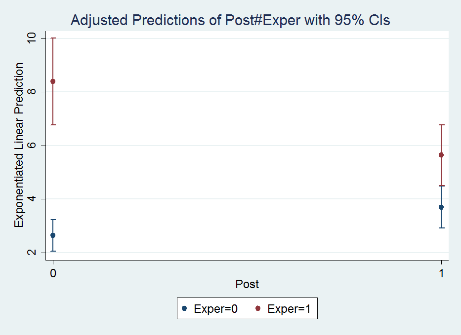
*Marginsplot
margins Post#Exper, at( (base) Month )
marginsplot, recast(scatter)

So basically once you estimate a regression equation, Stata has many of its attributes accessible to subsequent command. What the margins command does is predict the value of Y at the 2 by 2 factor levels for Post and Exper. The at( (base) Month ) option says to estimate the effects at the base level of the Month factor, which happens to default to January here. The marginsplot shows this easier than I can explain.

The option recast(scatter) draws the plot so there are no lines connecting the different points. Note I prefer to draw these error bar like plots without the end cross hairs, which can be done like marginsplot, recast(scatter) ciopts(recast(rspike)), but this causes a problem when the error bars overlap.

So I initially interpreted this simply as the experimental series went down by around 2 crimes, and the control series went up by around 1 crime. A colleague though pointed out the whole point of having control series though is to say what would have happend if the intervention did not take place (the counterfactual). Because the control series was going up, we would have also expected the experimental series to go up.

The coefficients in this model though don’t directly answer that question. To estimate that relative decrease is somewhat convoluted in this parameterization, but you can use the test and lincom post-estimation commands to do it. Test basically does linear model restrictions for one or multiple variables. This can be useful to test if multiple coefficients are equal to one another, or joint testing to see if one coefficient is equal to another, or to test if a coefficient is different from a non-zero value.

So to test the relative decrease in this DiD setup ends up being (which I am too lazy to explain):

test 1.Exper#1.Post = (1.Exper#0.Post + 0.Exper#1.Post)

Note you can also do a joint test for all dummy variables with testparm:

testparm i.Month

which spits out:

 ( 1)  2.Month = 0
 ( 2)  3.Month = 0
 ( 3)  4.Month = 0
 ( 4)  5.Month = 0
 ( 5)  6.Month = 0
 ( 6)  7.Month = 0
 ( 7)  8.Month = 0
 ( 8)  9.Month = 0
 ( 9)  10.Month = 0
 (10)  11.Month = 0
 (11)  12.Month = 0

           chi2( 11) =   61.58
         Prob > chi2 =    0.0000

The idea behind this is that it often does not make sense to test the significance of only one level of a dummy variable – you want to jointly test whether the whole set of dummy variables is statistically significant. Most of the time I do this using F-tests for model restrictions (see this example in R). But here Stata does a chi-square test. (I imagine they will result in the same inferences in most circumstances.)

test just gives inferential statistics though, I wanted an actual estimate of the relative decrease. To do this you can use lincom. So working with my same set of variables I get:

lincom 1.Exper#1.Post - 0.Exper#1.Post - 1.Exper#0.Post

Which produces in the output:

 ( 1)  - 0b.Exper#1.Post - 1.Exper#0b.Post + 1.Exper#1.Post = 0

------------------------------------------------------------------------------
           Y |      Coef.   Std. Err.      z    P>|z|     [95% Conf. Interval]
-------------+----------------------------------------------------------------
         (1) |  -.7367337   .1080418    -6.82   0.000    -.9484917   -.5249757
------------------------------------------------------------------------------

I avoid explaining why this particular set of coefficient contrasts produces the relative decrease of interest because there is an easier way to specify the DiD model to get this coefficient directly (see the Wikipedia page linked earlier for an explanation):

*An easier way to estimate the model
xtgee Y i.Exper i.Post Exper#Post i.Month, family(poisson) corr(ar1)

Which you can look at the output and see that the interaction term now recreates the same -.7367337 (.1080418) estimate as the prior lincom command:

Iteration 1: tolerance = .00065297
Iteration 2: tolerance = 1.375e-06
Iteration 3: tolerance = 2.682e-09

GEE population-averaged model                   Number of obs      =       264
Group and time vars:             Exper Ord      Number of groups   =         2
Link:                                  log      Obs per group: min =       132
Family:                            Poisson                     avg =     132.0
Correlation:                         AR(1)                     max =       132
                                                Wald chi2(14)      =    334.52
Scale parameter:                         1      Prob > chi2        =    0.0000

------------------------------------------------------------------------------
           Y |      Coef.   Std. Err.      z    P>|z|     [95% Conf. Interval]
-------------+----------------------------------------------------------------
     1.Exper |   1.157615   .0803121    14.41   0.000     1.000206    1.315023
      1.Post |    .339348   .0898574     3.78   0.000     .1632307    .5154653
             |
  Exper#Post |
        1 1  |  -.7367337   .1080418    -6.82   0.000    -.9484917   -.5249757
             |
       Month |
          2  |    .214908   .1243037     1.73   0.084    -.0287228    .4585388
          3  |   .2149183   .1264076     1.70   0.089    -.0328361    .4626726
          4  |   .3119988   .1243131     2.51   0.012     .0683497    .5556479
          5  |   .4416236   .1210554     3.65   0.000     .2043594    .6788877
          6  |    .556197   .1184427     4.70   0.000     .3240536    .7883404
          7  |   .4978252   .1197435     4.16   0.000     .2631322    .7325182
          8  |   .2581524   .1257715     2.05   0.040     .0116447      .50466
          9  |    .222813   .1267606     1.76   0.079    -.0256333    .4712592
         10  |    .430002    .121332     3.54   0.000     .1921956    .6678084
         11  |   .0923395   .1305857     0.71   0.479    -.1636037    .3482828
         12  |  -.1479884   .1367331    -1.08   0.279    -.4159803    .1200035
             |
       _cons |   .9699886   .1140566     8.50   0.000     .7464418    1.193536
------------------------------------------------------------------------------

But we can do some more here, and figure out the hypothetical experimental mean if the experimental series would have followed the same trend as the control series. Here I use nlcom and exponentiate the results to get back on the original count scale:

nlcom exp(_b[1.Exper] + _b[1.Post]  + _b[_cons])

Which gives an estimate of:

       _nl_1:  exp(_b[1.Exper] + _b[1.Post]  + _b[_cons])

------------------------------------------------------------------------------
           Y |      Coef.   Std. Err.      z    P>|z|     [95% Conf. Interval]
-------------+----------------------------------------------------------------
       _nl_1 |   11.78646   1.583091     7.45   0.000     8.683656    14.88926
------------------------------------------------------------------------------

So in our couterfactual world, the intervention decreased crimes from around 12 to 6 per month instead of 8 to 6 in my original interpretation, a larger effect because of the control series. We can show how nlcom reproduces the output of margins by reproducing the experimental series mean at the baseline, over 8 crimes per month.

*This creates the observed estimates, (at January) - if you want for another month need to add to above
margins Post#Exper, at( (base) Month )
*to show it recreates margins of pre period
nlcom exp(_b[1.Exper] + _b[_cons])

Which produces the output:

. margins Post#Exper, at( (base) Month )

Adjusted predictions                              Number of obs   =        264
Model VCE    : Conventional

Expression   : Exponentiated linear prediction, predict()
at           : Month           =           1

------------------------------------------------------------------------------
             |            Delta-method
             |     Margin   Std. Err.      z    P>|z|     [95% Conf. Interval]
-------------+----------------------------------------------------------------
  Post#Exper |
        0 0  |   2.637914   .3008716     8.77   0.000     2.048217    3.227612
        0 1  |   8.394722   .8243735    10.18   0.000      6.77898    10.01046
        1 0  |   3.703716   .3988067     9.29   0.000     2.922069    4.485363
        1 1  |   5.641881   .5783881     9.75   0.000     4.508261    6.775501
------------------------------------------------------------------------------

. *to show it recreates margins of pre period
. nlcom exp(_b[1.Exper] + _b[_cons])

       _nl_1:  exp(_b[1.Exper] + _b[_cons])

------------------------------------------------------------------------------
           Y |      Coef.   Std. Err.      z    P>|z|     [95% Conf. Interval]
-------------+----------------------------------------------------------------
       _nl_1 |   8.394722   .8243735    10.18   0.000      6.77898    10.01046
------------------------------------------------------------------------------

Poisson models are no big deal

Much of my experience suggests that although Poisson models are standard fare for predicting low crime counts in our field, they almost never make a difference when evaluating the marginal effects like I have above. So here we can reproduce the same GEE model, but instead of Poisson have it be a linear model. Here I use the quietly command to suppress the output of the model. Comparing coefficients directly between the two models does not make sense, but comparing the predictions is fine.

*Compare Poisson to a linear model
quietly xtgee Y Exper#Post i.Month, family(gaussian) corr(ar1)
margins Post#Exp, at( (base) Month )

And this subsequently produces:

Adjusted predictions                              Number of obs   =        264
Model VCE    : Conventional

Expression   : Linear prediction, predict()
at           : Month           =           1

------------------------------------------------------------------------------
             |            Delta-method
             |     Margin   Std. Err.      z    P>|z|     [95% Conf. Interval]
-------------+----------------------------------------------------------------
  Post#Exper |
        0 0  |   1.864656   .6951654     2.68   0.007     .5021569    3.227155
        0 1  |   9.404887   .6951654    13.53   0.000     8.042388    10.76739
        1 0  |   3.233312   .6992693     4.62   0.000     1.862769    4.603854
        1 1  |   5.810809   .6992693     8.31   0.000     4.440266    7.181351
------------------------------------------------------------------------------

The predictions are very similar between the two models. I simply state this here because I think the parallel trends assumption for the DiD model makes more sense on a linear scale than it does for the exponential scale. Pretty much wherever I look, the effects of explanatory variables appear pretty linear to me when predicting crime counts, so I think linear models make a lot of sense, even if you are predicting low count data, despite current conventions in the field.

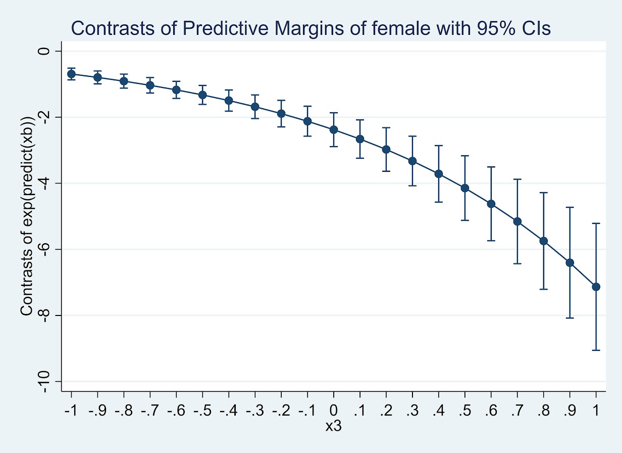
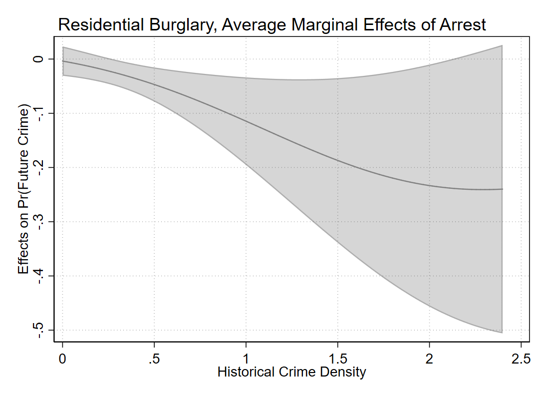
An additional Example using marginsplot and areas

Long post – but stick with me! The last thing I wanted to go over was how to get area’s instead of error bars for marginsplot. The pdf help online has some examples – so this is pretty much just a restatement of the help. (Stata’s help in the online PDFs are excellent – code and math and figures and references and intelligible discussion all in one.) Like Andrew Gelman, I think the discrete bars are misleading when the sample locations are just arbitrary locations along a continuous function. I also think the areas look nicer, especially when the error bars overlap.

So using the same example from Dan Kahan, we first use drop _all to get rid of the prior panel data, then use import to load up the csv file.

*This clears the prior data.
drop _all 

*grab the csv data
import delimited gelman_cup_graphic_reporting_challenge_data

Now we can estimate our model and our margins:

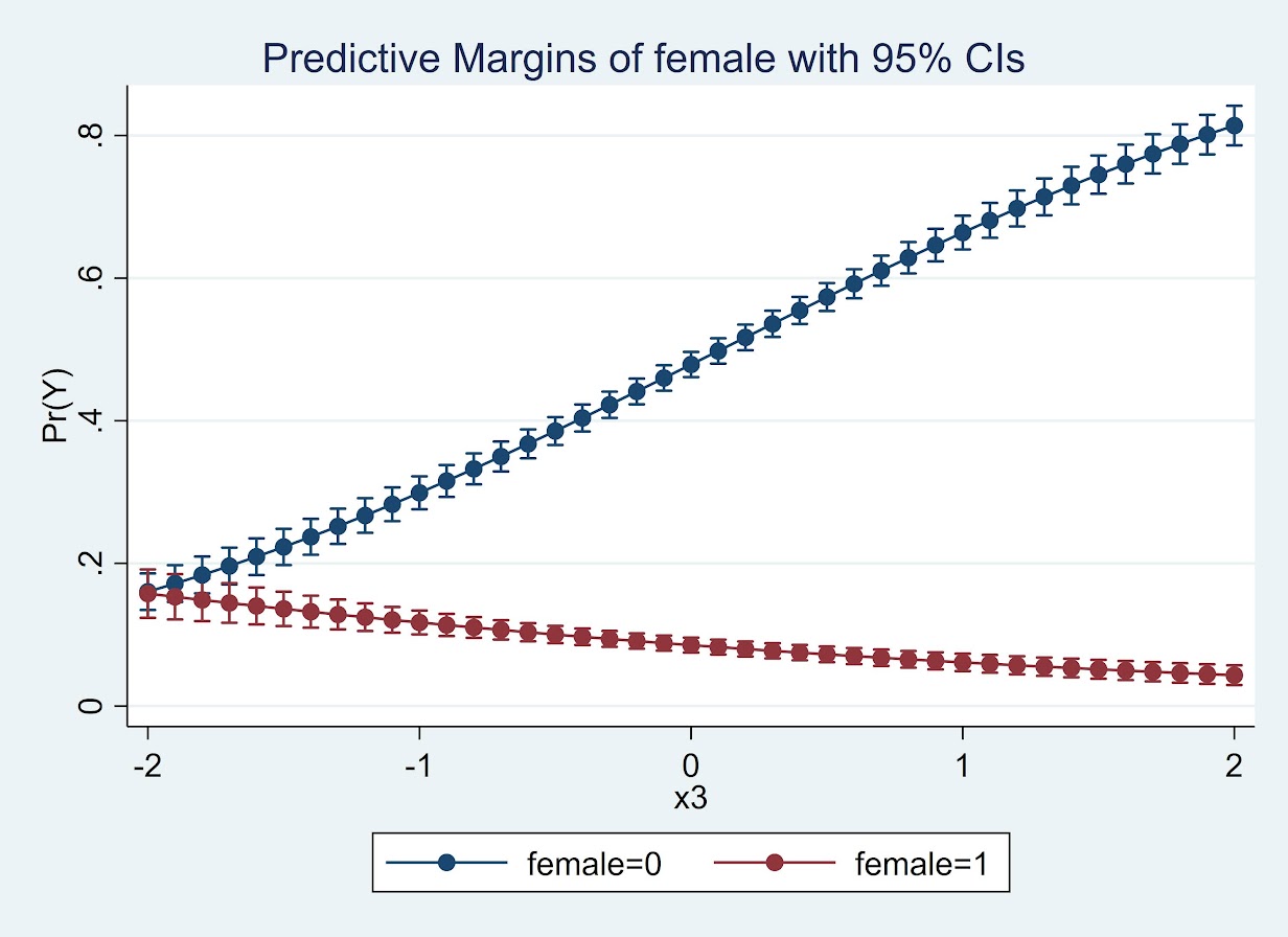
*estimate a similar logit model
logit agw c.left_right##c.religiosity
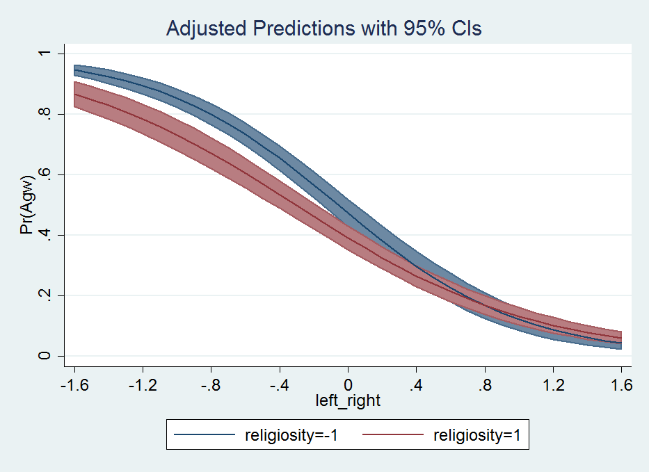
*graph areas using margins - pretended -1 and 1 are the high/low religious cut-offs
quietly margins, at(left_right=(-1.6(0.1)1.6) religiosity=(-1 1))

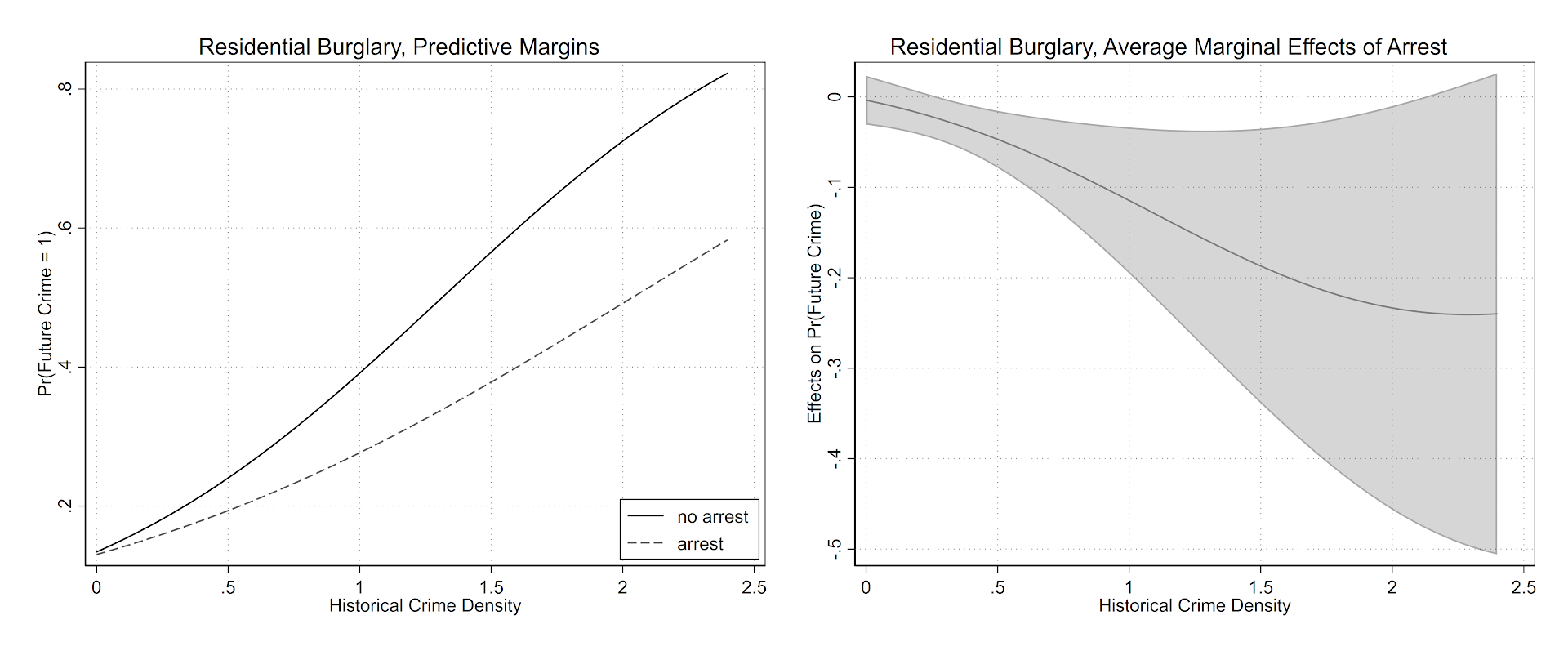
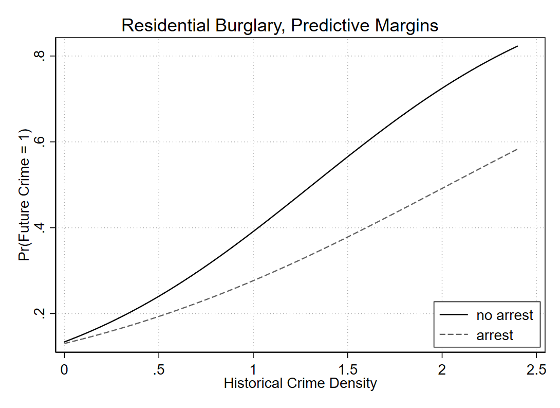
quietly is definately useful here for the margins command, we don’t want to pour through the whole text table, since it is only intended for a chart. And now to make our area chart at the sample points:

marginsplot, xlabel(-1.6(0.4)1.6) recast(line) recastci(rarea) ciopts(color(*.8))

That is much better looking that the default with the ugly cross-hair error bars overlapping. Stata draws the lines unfortunately in the wrong order (see the blue line over the red area), and if I figure out an easy way to fix that I will update the post in the future. I need to learn the options for Stata charts to a greater extent before I give any more advice about Stata charts though.

To wrap up. I typically have in my Stata do file:

**************.
*Finish the script.
drop _all 
exit, clear
**************.

This drops the dataset (as mentioned before), and exit, clear then basically closes out of Stata.

4 Comments

by apwheele on May 12, 2016 • Permalink

Posted in Data Visualization, Stata

Tagged panel-data, Stata

Posted by apwheele on May 12, 2016

https://andrewpwheeler.com/2016/05/12/some-stata-notes-difference-in-difference-models-and-postestimation-commands/

Search for:
Recent Posts
Categories
Categories
Site RSS Feeds
- RSS - Posts
- RSS - Comments
Follow Blog via Email

Enter your email address to follow this blog and receive notifications of new posts by email.

Email Address:

Join 328 other subscribers
aoristic big-data cartography census choropleth citeulike color cost-benefit courses crime-mapping crime-trends Crime Analysis Criminal Justice data-manipulation data visualization deep-learning excel flow-data geocoding ggplot2 github grammar of graphics group-based-trajectory gun-violence healthcare homicide-rates hot spots hypothesis-testing kernel-density linear programming logistic-regression machine-learning MACRO mapping matplotlib meta multi-level negative-binomial network NetworkX officer-involved-shooting open-science paper Papers peer-review Poisson prediction Predictive-Policing presentation Python Python-programability pytorch quasi-experiment r recidivism regression resources scatterplot scholarly seaborn shootings simulation slopegraph small-multiples social-networking SPSS stackexchange Stata statistics survey time-series uncertainty wdd web-scraping writing
Top Posts & Pages
Stack Exchange

All posts in category Stata

Example Linear Spline

Start Up

Graph Settings

Data Prep

Making a Nice marginsplot

SPSS

R

Stata

Codebook

Recent Posts

Categories

Site RSS Feeds

Follow Blog via Email

Top Posts & Pages

Stack Exchange