
As promised earlier, here is one example of testing coefficient equalities in SPSS, Stata, and R.
Here we have different dependent variables, but the same independent variables. This is taken from Dallas survey data (original data link, survey instrument link), and they asked about fear of crime, and split up the questions between fear of property victimization and violent victimization. Here I want to see if the effect of income is the same between the two. People in more poverty tend to be at higher risk of victimization, but you may also expect people with fewer items to steal to be less worried. Here I also control for the race and the age of the respondent.
The dataset has missing data, so I illustrate how to select out for complete case analysis, then I estimate the model. The fear of crime variables are coded as Likert items with a scale of 1-5, (higher values are more safe) but I predict them using linear regression (see the Stata code at the end though for combining ordinal logistic equations using suest). Race is of course nominal, and income and age are binned as well, but I treat the income bins as a linear effect. I pasted the codebook for all of the items at the end of the post.
These models with multiple dependent variables have different names, economists call them seemingly unrelated regression, psychologists will often just call them multivariate models, those familiar with structural equation modeling can get the same results by allowing residual covariances between the two outcomes — they will all result in the same coefficient estimates in the end.
SPSS
In SPSS we can use the GLM procedure to estimate the model. Simultaneously we can specify particular contrasts to test whether the income coefficient is different for the two outcomes.
*Grab the online data.
SPSSINC GETURI DATA URI="https://dl.dropbox.com/s/r98nnidl5rnq5ni/MissingData_DallasSurv16.sav?dl=0" FILETYPE=SAV DATASET=MissData.
*Conducting complete case analysis.
COUNT MisComplete = Safety_Violent Safety_Prop Gender Race Income Age (MISSING).
COMPUTE CompleteCase = (MisComplete = 0).
FILTER BY CompleteCase.
*This treats the different income categories as a continuous variable.
*Can use GLM to estimate seemingly unrelated regression in SPSS and test.
*equality of the two coefficients.
GLM Safety_Violent Safety_Prop BY Race Age WITH Income
/DESIGN=Income Race Age
/PRINT PARAMETER
/LMATRIX Income 1
/MMATRIX ALL 1 -1.
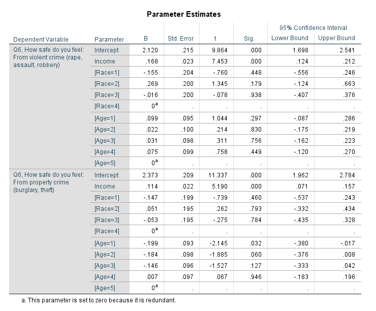
FILTER OFF. In the output you can see the coefficient estimates for the two equations. The income effect for violent crime is 0.168 (0.023) and for property crime is 0.114 (0.022).
And then you get a separate table for the contrast estimates.
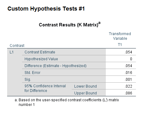
You can see that the contrast estimate, 0.054, equals 0.168 – 0.114. The standard error in this output (0.016) takes into account the covariance between the two estimates. Here you would reject the null that the effects are equal across the two equations, and the effect of income is larger for violent crime. Because higher values on these Likert scales mean a person feels more safe, this is evidence that those with higher incomes are more likely to be fearful of property victimization, controlling for age and race.
Unfortunately the different matrix contrasts are not available in all the different types of regression models in SPSS. You may ask whether you can fit two separate regressions and do this same test. The answer is you can, but that makes assumptions about how the two models are independent — it is typically more efficient to estimate them at once, and here it allows you to have the software handle the Wald test instead of constructing it yourself.
R
As I stated previously, seemingly unrelated regression is another name for these multivariate models. So we can use the R libraries systemfit to estimate our seemingly unrelated regression model, and then use the library multcomp to test the coefficient contrast. This does not result in the exact same coefficients as SPSS, but devilishly close. You can download the csv file of the data here.
library(systemfit) #for seemingly unrelated regression
library(multcomp) #for hypothesis tests of models coefficients
#read in CSV file
SurvData <- read.csv(file="MissingData_DallasSurvey.csv",header=TRUE)
names(SurvData)[1] <- "Safety_Violent" #name gets messed up because of BOM
#Need to recode the missing values in R, use NA
NineMis <- c("Safety_Violent","Safety_Prop","Race","Income","Age")
#summary(SurvData[,NineMis])
for (i in NineMis){
SurvData[SurvData[,i]==9,i] <- NA
}
#Making a complete case dataset
SurvComplete <- SurvData[complete.cases(SurvData),NineMis]
#Now changing race and age to factor variables, keep income as linear
SurvComplete$Race <- factor(SurvComplete$Race, levels=c(1,2,3,4), labels=c("Black","White","Hispanic","Other"))
SurvComplete$Age <- factor(SurvComplete$Age, levels=1:5, labels=c("18-24","25-34","35-44","45-54","55+"))
summary(SurvComplete)
#now fitting seemingly unrelated regression
viol <- Safety_Violent ~ Income + Race + Age
prop <- Safety_Prop ~ Income + Race + Age
fitsur <- systemfit(list(violreg = viol, propreg= prop), data=SurvComplete, method="SUR")
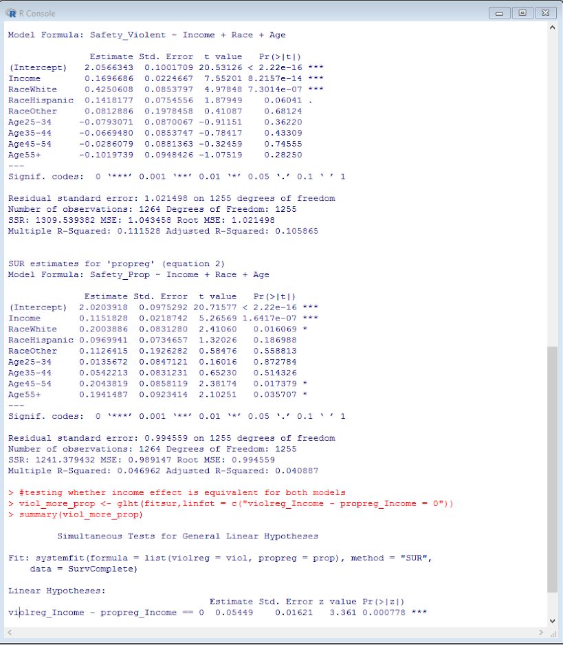
summary(fitsur)
#testing whether income effect is equivalent for both models
viol_more_prop <- glht(fitsur,linfct = c("violreg_Income - propreg_Income = 0"))
summary(viol_more_prop) Here is a screenshot of the results then:
This is also the same as estimating a structural equation model in which the residuals for the two regressions are allowed to covary. We can do that in R with the lavaan library.
library(lavaan)

#for this need to convert factors into dummy variables for lavaan
DumVars <- data.frame(model.matrix(~Race+Age-1,data=SurvComplete))
names(DumVars) <- c("Black","White","Hispanic","Other","Age2","Age3","Age4","Age5")

SurvComplete <- cbind(SurvComplete,DumVars)

model <- '
    #regressions
     Safety_Prop    ~ Income + Black + Hispanic + Other + Age2 + Age3 + Age4 + Age5
     Safety_Violent ~ Income + Black + Hispanic + Other + Age2 + Age3 + Age4 + Age5
    #residual covariances
     Safety_Violent ~~ Safety_Prop
     Safety_Violent ~~ Safety_Violent
     Safety_Prop ~~ Safety_Prop
'

fit <- sem(model, data=SurvComplete)
summary(fit)
I’m not sure offhand though if there is an easy way to test the coefficient differences with a lavaan object, but we can do it manually by grabbing the variance and the covariances. You can then see that the differences and the standard errors are equal to the prior output provided by the glht function in multcomp.
#Grab the coefficients I want, and test the difference
PCov <- inspect(fit,what="vcov")
PEst <- inspect(fit,what="list")
Diff <- PEst[9,'est'] - PEst[1,'est']
SE <- sqrt( PEst[1,'se']^2 + PEst[9,'se']^2 - 2*PCov[9,1] )
Diff;SE
Stata
In Stata we can replicate the same prior analyses. Here is some code to simply replicate the prior results, using Stata’s postestimation commands (additional examples using postestimation commands here). Again you can download the csv file used here. The results here are exactly the same as the R results.
*Load in the csv file
import delimited MissingData_DallasSurvey.csv, clear

*BOM problem again
rename ïsafety_violent safety_violent

*we need to specify the missing data fields.
*for Stata, set missing data to ".", not the named missing value types.
foreach i of varlist safety_violent-ownhome {
    tab `i'
}

*dont specify district
mvdecode safety_violent-race income-age ownhome, mv(9=.)
mvdecode yearsdallas, mv(999=.)

*making a variable to identify the number of missing observations
egen miscomplete = rmiss(safety_violent safety_prop race income age)
tab miscomplete
*even though any individual question is small, in total it is around 20% of the cases

*lets conduct a complete case analysis
preserve
keep if miscomplete==0

*Now can estimate multivariate regression, same as GLM in SPSS
mvreg safety_violent safety_prop = income i.race i.age

*test income coefficient is equal across the two equations
lincom _b[safety_violent:income] - _b[safety_prop:income]

*same results as seemingly unrelated regression
sureg (safety_violent income i.race i.age)(safety_prop income i.race i.age)

*To use lincom it is the exact same code as with mvreg
lincom _b[safety_violent:income] - _b[safety_prop:income]

*with sem model
tabulate race, generate(r)
tabulate age, generate(a)
sem (safety_violent <- income r2 r3 r4 a2 a3 a4 a5)(safety_prop <- income r2 r3 r4 a2 a3 a4 a5), cov(e.safety_violent*e.safety_prop)

*can use the same as mvreg and sureg
lincom _b[safety_violent:income] - _b[safety_prop:income]
You will notice here it is the exact some post-estimation lincom command to test the coefficient equality across all three models. (Stata makes this the easiest of the three programs IMO.)
Stata also allows us to estimate seemingly unrelated regressions combining different generalized outcomes. Here I treat the outcome as ordinal, and then combine the models using seemingly unrelated regression.
*Combining generalized linear models with suest
ologit safety_violent income i.race i.age
est store viol

ologit safety_prop income i.race i.age
est store prop

suest viol prop

*lincom again!
lincom _b[viol_safety_violent:income] - _b[prop_safety_prop:income]
An application in spatial criminology is when you are estimating the effect of something on different crime types. If you are predicting the number of crimes in a spatial area, you might separate Poisson regression models for assaults and robberies — this is one way to estimate the models jointly. Cory Haberman and Jerry Ratcliffe have an application of this as well estimate the effect of different crime types at different times of day – e.g. the effect of bars in the afternoon versus the effect of bars at nighttime.
Codebook
Here is the codebook for each of the variables in the database.
Safety_Violent
    1   Very Unsafe
    2   Unsafe
    3   Neither Safe or Unsafe
    4   Safe
    5   Very Safe
    9   Do not know or Missing
Safety_Prop
    1   Very Unsafe
    2   Unsafe
    3   Neither Safe or Unsafe
    4   Safe
    5   Very Safe
    9   Do not know or Missing
Gender
    1   Male
    2   Female
    9   Missing
Race
    1   Black
    2   White
    3   Hispanic
    4   Other
    9   Missing
Income
    1   Less than 25k
    2   25k to 50k
    3   50k to 75k
    4   75k to 100k
    5   over 100k
    9   Missing
Edu
    1   Less than High School
    2   High School
    3   Some above High School
    9   Missing
Age
    1   18-24
    2   25-34
    3   35-44
    4   45-54
    5   55+
    9   Missing
OwnHome
    1   Own
    2   Rent
    9   Missing
YearsDallas
    999 Missing

M Zargar
/ August 8, 2017What about in a multinomial logistic regression? How would you test the significance of the difference between the coefficients of an IV on the different levels of DV? Let’s say we are seeking to understand the effect of IV on levels 1 and 2 of DV (level 0 is the baseline). Is there a way we can compare the two coefficients we obtain for the IV?
apwheele
/ August 8, 2017Excellent example use – in multinomial you just get the coefficients relative to the baseline category, but you often want to test the coefficients against multiple categories. Testing one coefficient against another works very similar – you just need to covariance between those two estimates to formulate the test statistic of the difference.
In multinomial though you may want a global test whether a covariate has any effect over all of the dependent variable categories. For that you can either do an F test (with and without that variable), or adapt the Wald test to multivariate data.
I will need to do another blog post! See here for a good example in Stata, https://stats.idre.ucla.edu/stata/dae/multinomiallogistic-regression/, I will need to see if you can easily do those tests in SPSS and R though.
M Zargar
/ August 9, 2017I followed the instructions on the IDRE website, and it was quite easy on STATA to do the tests, but then I couldn’t figure it out on R (the equivalent IDRE R page on multinomials doesn’t include them). But thanks to a benevolent contributor on CrossValidated (wink wink), I have the answer now!
RC2223
/ April 17, 2018Thank you so much for this helpful post. Is there a chance that the analyses above could be done on multiply imputed data in R (and provide a pooled result)? I am hoping to use systemfit’s SUR function but pooling those output has proven to be a major challenge. I imagine that Lavaan might better handle imputed data but overall the output does not seem to be as streamlined.
apwheele
/ April 18, 2018This is actually what I have my students do in one of my classes. It is a bit of work in R (easier in Stata), but in the zip file in the link there is R code showing how to do this with multiple imputation using systemfit. Also includes Stata code (and SPSS, but I see I don’t have code to pool the results in SPSS).
https://www.dropbox.com/s/f86ugqr08n0345l/9_MissingData_Analysis.zip?dl=0
RC2223
/ April 18, 2018Wow. This is INCREDIBLE help. Thank you!!!
Antonio222
/ January 26, 2019In Stata, why do you use “lincom” and not “test”?
apwheele
/ January 26, 2019Test you just get the p-value, whereas lincom you get an estimate of the size of the difference. For single tests they will be the same anyway, but if you want to do several hypothesis tests at once you can do that via test.
Alexander
/ February 7, 2019For the lavaan example, I believe you could define a simple contrast in your model to get estimates of equivalence. This would be something like “contrast := Safety_Prop – Safety_Violent” in your example. (The screenshots are alas dead in your post, so I cannot verify if it really gives identical estimates or not, but it seems to work on my data).
apwheele
/ February 7, 2019Good call, you can name the coefficients in the lavaan model object and then do the contrast. So this works and does give the same estimates for `inc_cont`
mcont <- '
#regressions
Safety_Prop ~ b1*Income + Black + Hispanic + Other + Age2 + Age3 + Age4 + Age5
Safety_Violent ~ b2*Income + Black + Hispanic + Other + Age2 + Age3 + Age4 + Age5
#residual covariances
Safety_Violent ~~ Safety_Prop
Safety_Violent ~~ Safety_Violent
Safety_Prop ~~ Safety_Prop
#contrast
inc_cont := b2 – b1
'
Screenshots hopefully work now, not sure what happened there. If you see other posts with missing screen shots let me know please!
Camila
/ March 30, 2020This is a very helpful article. However I still wonder how to test whether one coefficient is larger than the other, i. e. to employ a one-tailed test, e. g. using suest from STATA.
apwheele
/ March 30, 2020Mathematically it would if be a conditional function, so if you are testing if something is greater than:
if Ha > Ho: “two-tailed p-value” * 2 = “one-tailed p-value”
else: 1 – (“two-tailed p-value”*2) = “one-tailed p-value”
There is probably a flag to do this in Stata, but I don’t know it offhand.
(((Sam Leighton))) (@samleighton87)
/ May 10, 2020Thank you for a wonderful explanation. I am not a statistician but a physician so trying to understand as best I can. Apologies in advance.
I had a question regarding the R analysis.
Does the following:
viol <- Safety_Violent ~ Income + Race + Age
prop <- Safety_Prop ~ Income + Race + Age
fitsur <- systemfit(list(violreg = viol, propreg= prop), data=SurvComplete, method="SUR")
summary(fitsur)
Do the same thing as:
fitsur <- lm(cbind(Safety_Violent, Safety_Prop) ~ Income + Race + Age))
summary(fitsur)
Also, would the contrasts be considered an appropriate post-hoc test to a type ii manova? I.e. if one did the following:
car::Anova(modelFit_both_death_all)
If so, can the contrast:
viol_more_prop <- glht(fitsur,linfct = c("violreg_Income – propreg_Income = 0"))
summary(viol_more_prop)
be done using the car::linearHypothesis() method?
Thanks,
Sam
apwheele
/ May 10, 2020Here they are equivalent because the cross-equations all contain the same right hand side variables (so estimating all at once is just a convenience — they can be estimated separately and get the same results).
That is the first time I have seen cbind being used like that — so that is new to me. (I’ve seen it used like that for binomial outcomes of numerator/denominator.) It isn’t clear to me that when you do that R estimates the covariance matrix of the residuals, which will alter the coefficients/standard errors downstream for any post-hoc test.
I imagine there is a way to get the same info from manova or the car package — I don’t know for R though offhand (you can see I did that in the SPSS/Stata code).
(((Sam Leighton))) (@samleighton87)
/ May 10, 2020sorry made a slight error in my code:
lm(cbind(Safety_Violent, Safety_Prop) ~ Income + Race + Age), data = data)
missed the data argument – the rest are variables
(((Sam Leighton))) (@samleighton87)
/ May 10, 2020I suppose I wanted to know if a coefficients was both significantly different across the two models and against zero given the presence the of both dependent variables. In your method you could do separate glht tests for the coefficient against itself across the models and separately against zero. Manova would answer the against zero question I think. Please excuse my ignorance if I am getting this all wrong.
apwheele
/ May 10, 2020I mean you can do them separately — this just does it in one call. It doesn’t do any special multiple comparison adjustment though that I can tell (you might do that yourself?)
###########################
mult_test <- glht(fitsur,linfct = c("violreg_Income – propreg_Income = 0",
"violreg_Income=0",
"propreg_Income=0"))
summary(mult_test)
###########################
Veronica Martines
/ June 11, 2020Thank you so much for providing this very useful article. I wonder how I could run the same analysis in SPSS for a poison regression.
Santi Allende
/ March 29, 2021Thanks so much for this post! Would this work for instances where the models have different independent variables? I have 2 lme models that use the same data and have the same predictors, except for 2 that differ across models (anxiety and depression vars are switched as dependent and independent variables in models). i.e., depression ~ anxiety + anxietyLag(1) + sameCovariates vs. anxiety ~ depression + depressionLag(1) + sameCovariates. I’d like to test anxietyLag(1) vs. depressionLag(1). Thank you!
apwheele
/ March 29, 2021It is mostly ok in this scenario — with one caveat. Doing the estimate assumes a zero covariance between the two coefficients across the models, which with largish samples (say over 1000 observations) is typically not a real onerous assumption. You could estimate this covariance by either stacking the models or estimating a seemingly unrelated regression.
A bigger issue as stated IMO is bias in the coefficients themselves. Not 100% clear if your equations are endogenous that you have unbiased estimates for the non-lagged effects (which I presume can also bias the lagged effects).
Emily
/ April 28, 2021Thank you so much– this is SO useful! I used the R code and got it to work (although FYI I needed to add formula() around the regression formulas to get them to work with systemfit()). Do you know if it’s OK to do SUR on negative binomial models? Thanks again!
apwheele
/ April 28, 2021I would check out Stata maybe to see if you can use the suest command like I show with the ordered logit. Not 100% sure — main thing I am not sure about is how the dispersion term is handled (but you can use it with Poisson, which should result in very similar inferences).
Another approach is to stack the data and estimate a single equation, but there again with negative binomial you have the issue of whether to let the dispersion term vary across the dependent variables or constrain them to be the same.
Emily
/ April 28, 2021OK, thanks so much!!
Gebretsadik shibre
/ July 1, 2022Dear,
Thanks so much. The post is very useful. One thing I cannot understand is how can we test the equality of coefficients of a categorical variable across 3 or more time periods?
I want to check or test whether the effect of a categorical variable change over time in 2000, 2005 and 2011 DHS data. the categorical variable is education ( 4 categories) and the time has 3 categories (2000, 2005 and 2011)., and my outcome variable is service use. Now, can I test the effect of education as a whole or for its categories separately? How can I do this in stata?
Thanks in advance.
apwheele
/ July 1, 2022High level if you have 3 effects, say T1, T2, T3, you can then do 3 pairwise tests:
T1 vs T2
T1 vs T3
T2 vs T3
And then you need to worry about potential for multiple hypothesis testing, but just focusing on the magnitude of the differences is OK. Note here since you have temporal ordering, it may only make sense to both doing tests for consecutive periods, e.g. don’t worry about T1 vs T3.
Another approach though is to fit a restricted model, so say a single effect T without varying over time. And then do a likelihood ratio test of the restricted model vs the model with changes over time.
I prefer the approach fit a general model and then just describe differences over time. In Stata it may be something post reg (this just does the pairwise tests for each subsequent time period, broken down by education):
margins ar.time, over(i.edu)
See this post for several notes on doing different margins/contrasts post regression in Stata, https://andrewpwheeler.com/2021/06/28/marginal-effects-vs-wald-tests-stata/.
gebretsadikshibre
/ July 1, 2022Dear, thanks so much again. I really appreciate your very prompt and interesting response.
My intention in my study is to inlude interaction between education and year in my model. previously, I was thinking to just include year (to time of the survey) as fixed effect variable like any other variables. recently, however, I start thinking that ( after I read many sources) I must also allow the effect of educ
gebretsadikshibre
/ July 1, 2022Dear, Thanks so much again. I really appreciate your very prompt and interesting response.
My intention in my study is to include interaction between education and year in my model. previously, I was thinking to just include year (to time of the survey) as a fixed effect variable like any other variable. recently, however, I started thinking that (after I read many sources) I must also allow the effect of education to vary across time and thus include interaction terms in the model between education and year. However, I should not simply include this interaction without first checking whether education’s effect is constant over time or fixed. That is why I want to check whether its effect changes over time. If it does not change, then I will not include the interaction, but if its effect varies over time, then I will include the interaction.
Another related problem is, I tried to use lincom to test differences in effect of education across time, but I what this command does is it allows me to test only 2 coefficients at time for example category 1 in 2000 and category 1 in 2005,, and this difference may be significant. But for category 2 in 2000 and 2005, there might not be a difference. So, can I say that education varies over time when only some of its categories change over time but others do not?
For your information, my study focuses on pooled cross section that involves four DHS rounds, and I want to see whether education changes between 2000 and 2016.
Thanks and keep blessed.
apwheele
/ July 1, 2022So if you have a model that is something like
reg service_use i.edu##i.time
And lets say edu has 2 levels (highschool,college) and 3 time periods
your final model results could be something like:
effect HighSchool
period1 0.9
period2 0.7
period3 0.5
effect college
period1 0.9
period2 0.9
period3 0.9
etc. So here the effects of college over time are constant. But highschool has decreasing usage effects over time. Say service got more expensive, and so only marginally impacted those with lower edu because of cost.
Unless service use is 0 sum (e.g. if college goes up highschool has to go down), then it seems straightforward to me that some effects can vary and some can stay the same.
gebretsadikshibre
/ July 1, 2022Thank you so much, Dr.
gebretsadikshibre
/ July 3, 2022Dear Dr, thanks so much again.
I am now coming with a different question.’
I would like to model poisson regression for my binary outcome variable (whether or not women receive the service in 5 years time period using DHS data). I have decided to use poisson because logitic regression cannot answer my research question. So, my question is that should I include an offset variable in my model or not?
Regards,
apwheele
/ July 3, 2022Offset’s are typically used as denominators for rates for some time period. So if you have a field that measures the potential time period a women *could* have gotten the service, and that variable varies over women, then it might make sense.
For example, say it is marriage counseling. It would only make sense after they are married. So if you have a variable in the data “years married” and “did you get marriage counseling” you could argue to use log(years married) as an offset in Poisson regression. You can see my class notes on Poisson regression and offsets, https://apwheele.github.io/MathPosts/PoissonReg.html
gebretsadikshibre
/ July 12, 2022Dear Dr, I thank you for your useful assistance on our statistical practice. I would like to kindly drop a couple of questions for you to help me.
1). I am attempting to create a variable by combining existing variables. the existing variables in my dataset are education (no education=0, primary=1, secondary=2, or higher=3), wealth index (poorest=1, poorer=2, medium=3, rich=4, richest=5), and place of residence (urban=1, rural=2). I want to create a variable by multiplying all these variables (education*wealth*residence, 4*5*2, giving a variable with 40 categories. Now, my question is how do I label all of these 40 categories in STATA? For example, how do I know that a category with 0 is a result of no education (0) *poorest*rural? or no education (0) *poorest*urban?. Knowing which combinations gives which category is important to analyze the categories by their name. If I know that 0 in the category contains the poorest and non-educated people who live in urban area is different from that who lives in rural setting.
2). How do we compare 2 summary measures ( eg: concentration index ) for 2 time periods to see whether they changed statistically significantly? I cannot use conventional methods such as “lincom” to test the significance of the measures because these measures are not available in the form of coefficients or their exponentiated version. For example, in T1, I did a regression and got a summary value of 2 and of 4 in T2. Now, I wanted to test whether the difference between these two values is significant. Since I cannot store these values in Stata, I cannot use the software to test significance test.
Your assistance is always appreciated
Regards,
apwheele
/ July 12, 2022For 1 check out labels in Stata.
For 2 your description is too vague (and somewhat contradictory). If say we wanted to assess a continuous index in two periods for changes in two samples (the two periods), you could do a t-test, a KS test, other distribution test, etc.
You say you have coefficients though later in the description, then it would be the case to do the same Wald tests I describe in this post.
gebretsadikshibre
/ July 12, 2022Sorry dear Dr for the vague description of my question.
I just wanted to test the significance test of two summary values in two periods. In period 1, I calculated it to be 2 and in T2, it is 4. The index is simply the average gap between urban and rural settings in terms of service use.
Regards,
Mathieu
/ July 19, 2022Thank you very much for this wonderful post, it helped me a lot.
I was just wondering what formula the glht function in R uses exactly. Because my initial idea of approaching this issue was by just running OLS regressions on the two separate models and afterwards performing a z-test (are the coefficients of the variables from the two different regressions, which each have a certain standard error as well, the same?). However, this gives different results…
apwheele
/ July 19, 2022glht uses the same formulas I have provided to calculate the linear effect and its variance, although can be generalized to even more differences (e.g. you could do something like `b1 – b2 + 2*m3 = 0`).
The difference between glht (estimating your two equations at the same time) is that it allows R to calculate a covariance term between the two coefficients, whereas your “do two separate regressions” by itself there is no estimate of the covariance.
Mathieu
/ July 19, 2022Thank you for this clarification!
One follow-up question: the reason that I was interested in calculating the effect myself (based on two separate regressions), is that I want to correct the standard errors in the regressions for heteroskedasticity. Normally, I do this with ‘coeftest(output, vcov=vcovHC(output, type=”HC1″))’
Is there a way to do something similar with the glht command?
apwheele
/ July 19, 2022glht has an argument to pass in vcov the same as an argument.
Ano
/ November 15, 2022Thank you very much for your super helpful post!
I am sorry that I have to ask – maybe, it is very simple, but I tried a lot, and it did not work:
I also would like to correct the standard errors in the regressions for heteroskedasticity. Normally, I do it with summ(model, robust = “HC3”). For consistency, I would now like to apply HC3 also to the test of equality.
Applying your steps
#now fitting seemingly unrelated regression
viol <- Safety_Violent ~ Income + Race + Age
prop <- Safety_Prop ~ Income + Race + Age
fitsur <- systemfit(list(violreg = viol, propreg= prop), data=SurvComplete, method="SUR")
summary(fitsur)
#testing whether income effect is equivalent for both models
viol_more_prop <- glht(fitsur,linfct = c("violreg_Income – propreg_Income = 0"))
summary(viol_more_prop)
to my model works perfectly. However, how exactly can I include the HC3 correction?
apwheele
/ November 15, 2022The glht function you can pass in a variance/covariance matrix. So do not have code handy, but you can use the sandwich package to generate your robust variance/covariance matrix, and then pass that as an argument into glht.
gebretsadikshibre
/ November 16, 2022Thanks for the useful posts.
I would like to kindly ask a question:
I want to assess the discriminatory accuracy of my logistic regression model.
How could I assess whether my model accurately classifies cases from non-cases? In the literature, there is a suggestion to use ROC and the area under the ROC (auc). However, since I used pweght in my model, the Stata commands for computing ROC did not support pweight. How should I go about these issues?
Thanks in advance for your assistance.
Regards,
apwheele
/ November 16, 2022This doesn’t have anything to do with this post. I have posted other examples on this blog of using frequency weights with ROC curves (I presume using probability weights is feasible to figure out, even if Stata does not support it out of the box).
The first old Statalist post that comes up with some googling is fudging your pweights to make frequency weights, https://www.stata.com/statalist/archive/2009-01/msg00842.html. I don’t know if the ROC standard errors are still good using that, but the curve and AUC stat itself will be fine.
So you will just have to do some digging to figure out the best case for your scenario.
Jacob E
/ April 8, 2023Hi! Great walk-through and perfectly applicable to the problem I’m trying to solve at the moment with same independent but different dependent measures. I initially estimated the beta-coefficient seperately and calculated the Z-test, but this is much more elegant and accounts for the covariance. I was just wondering what your take is on the dependence between the observations since in this example it’s same individuals answering both dependent measures and whether this might disturb the results? Is this only valid when the two dependent measures are uncorrelated? Just now read an article on using GEE analysis for tackling correlated observations. I would be interested to hear your opinion on it. Thanks!
Yan, J., Aseltine, R., & Harel, O. (2013). Comparing Regression Coefficients Between Nested Linear Models for Clustered Data With Generalized Estimating Equations. Journal of Educational and Behavioral Statistics, 38(2), 172-189.
apwheele
/ April 8, 2023In this framework there is no extra within person variance, since you only have a single observation per person.
Now, say you asked the same survey instrument at two different occasion to the same individual. There is perhaps the territory you are getting into with the cited paper. You may either adjust the standard error estimates for the clustering, or you may wish to estimate contrasts for each group.
Imagine here instead of clustering for people, you clustered by neighborhood. And you then estimated a different contrast for each neighborhood via a multi-level model. That is a different approach than the “adjusting standard error” approach.
Tatja
/ September 4, 2024Thank you very much for this very useful article! How would I implement your example in R if I wanted to use Poisson regression instead of linear regression? Thanks again!
apwheele
/ September 4, 2024I would stack the data and estimate an interaction term. So something like:
“`
d1 <- SurvData[,c(“Safety_Violent”,”Income”,”Race”,”Age”)
d1$Type <- “Violent”
d2 <- SurvData[,c(“Safety_Prop”,”Income”,”Race”,”Age”)]
d2$Type <- “Property”
coln <- c(“Safety”,”Income”,”Race”,”Age”,”Type”)
names(d1) <- coln
names(d2) <- coln
stacked_data <- rbind(d1,d2)
reg <- glm(Safety ~ Type:(Income + Race + Age),family=”Poisson”)
“`