Calli Cain, a criminologist from FAU asks:
What is the best method to examine whether there are group differences (e.g., gender, race) in the effects of several variables on binary outcomes (using logistic regression)? For example – if you want to look at the gendered effects of different types of trauma experiences on subsequent adverse behaviors (e.g., whether participant uses drugs, alcohol, has mental health diagnosis, has attempted suicide). Allison (1999) cautions against using Equality of Coefficients tests to look at group differences between regression coefficients like we might with OLS regression. If you wanted to look at the differences between a lot of predictors (n= 16) on various outcomes (n=6) – what would be best way to go about it (I know using interaction terms would be good if you were just interested in say gender differences of one or two variables on the outcome). Someone recommended comparing marginal effects through average discrete changes (ADCs) or discrete changes at representative values (DCRs) – which is new to me. Would you agree with this suggestion?
When I am thinking about should I use method X or method Y type problems, I think about the specific value I want to estimate first, and then work backwards about the best method to use to get that estimate. So if we are talking about binary endpoints such as uses drugs (will go with binary for now, but my examples will readily extend to say counts or real valued outcomes), there are only generally two values people are interested in; say the change in probability is 5% given some input (absolute risk change, e.g. 10% to 5%), or a relative risk change such as X decreases the overall relative risk by 20% (e.g. 5% to 4%).
The former, absolute change in probabilities, is best accomplished via various marginal effects or average discrete changes as Calli says. Most CJ examples I am aware of I think these make the most sense to focus on, as they translate more directly to costs and benefits. Focusing on the ratio’s sometimes makes sense, such as in case-control studies, or if you want to extrapolate coefficient estimates to a very different sample. Or if you are hyper focused on theory and the underlying statistical model.
Will show an example in Stata using simulated data to illustrate the differences. Stata is very nice to work with different types of marginal estimates. Here I generate data with three covariates, female/males, and then some interactions. Note the covariate x1 has the same effect for males/females, x2 and x3 though have countervailing effects (females it decreases, males it increases the probability).
* Stata simulation to show differences in Wald vs Margins
clear
set more off
set seed 10
set obs 5000
generate female = rbinomial(1,0.5)
generate x1 = rnormal(0,1)
generate x2 = rnormal(0,1)
generate x3 = rnormal(0,1)

* x1 same effect, x2/x3 different across groups
generate logit = -0.1 + -2.8*female + 1.1*(x1 + x2 + x3) + -1.5*female*(x2 + x3)
generate prob = 1/(1 + exp(-1*logit))
generate y = rbinomial(1,prob)
drop logit prob
I intentionally generated the groups so females/males have quite different baseline probabilities for the outcome y here – something that happens in real victim data in criminology.
* Check out marginal differences
tabstat y, by(female)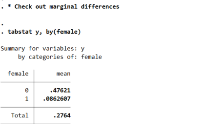
So you can see males have the proportion of the outcome near 50% in the sample, whereas females are under 10%. So Calli is basically interested in the case below, where we estimate all pairwise interactions, so have many coefficient differences to test on the right hand side.
* Estimate model with interactions (linear coefficients)
logistic y i.female x1 x2 x3 i.female#(c.x1 c.x2 c.x3), coef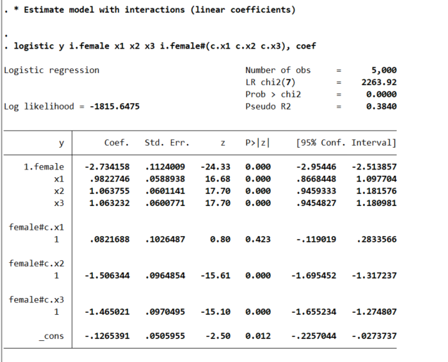
This particular model does the Wald tests for the coefficient differences just by the way we have set up the model. So the interaction effects test for differences from the baseline model, so can see the interaction for x1 is not stat significant, but x2/x3 are (as they should be). But if you are interested in the marginal effects, one place to start is with derivatives directly, and Stata automatically for logit models spits out probabilities:
* Marginal effects
margins female, dydx(x1 x2 x3)
* x1 is the same linear effect, but margins are quite different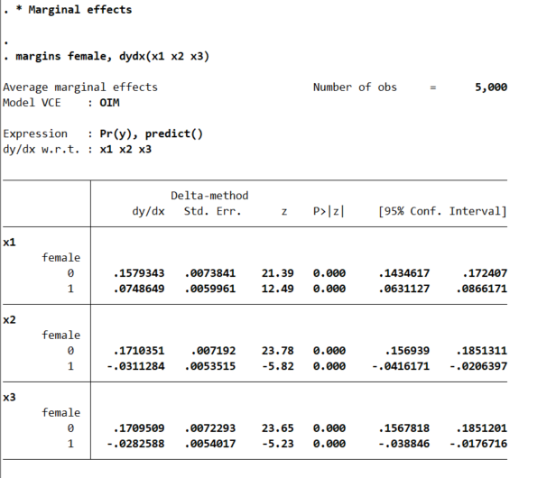
So even though I made the underlying effect for x1 equal between males/females for the true underlying data generation process, you can see here the marginal derivative is much smaller for females. This is the main difference between Wald tests and margins.
This is ok though for many situations. Say x1 is a real valued treatment, such as Y is victimization in a sample of high risk youth, and x1 is hours given for a summer job. We want to know the returns of expanding the program – here the returns are higher for males than females due to the different baseline probabilities of risk between the two. This is true even if the relative effect of summer job hours is the same between the two groups.
Again Stata is very convenient, and we can test for the probability differences in males/females by appending r. to the front of the margins command.
* can test difference contrast in groups
margins r.female, dydx(x1 x2 x3)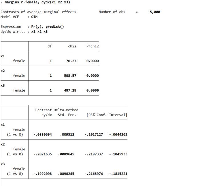
But the marginal derivative can be difficult to interpret – it is the average slope, but what does that mean exactly? So I like evaluating at fixed points of the continuous variable. Going back to our summer job hours example, you could evaluate going from 0 to 50 hours, or going from 50 to 100, or 0 to 100, etc. and see the average returns in terms of reductions in the probability of trauma. Here because I simulated the data to be a standard normal, I just go from -1 to 0 to 1:
* Probably easier to understand at particular x1 values
margins female, at(x1=(-1(1)1))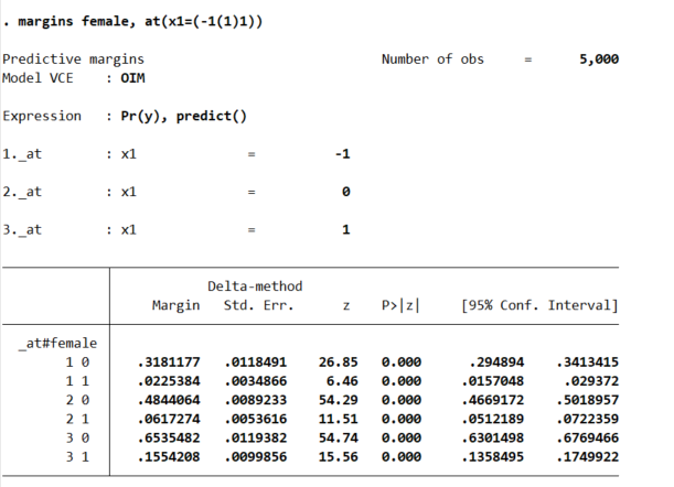
So that table is dense, but it says when x1=-1, females have a probability of y of 2%, and males have a probability of y of 32%. Now go up the ladder to x1=0, females have a probability of 6% and males have a probability of 48%. So a discrete change of 4% for females and 16% for males. If we want to generate an interval around that discrete change effect:
* Can test increases one by one
margins female, at(x1=(-1 0 1))   contrast(atcontrast(ar) effects marginswithin)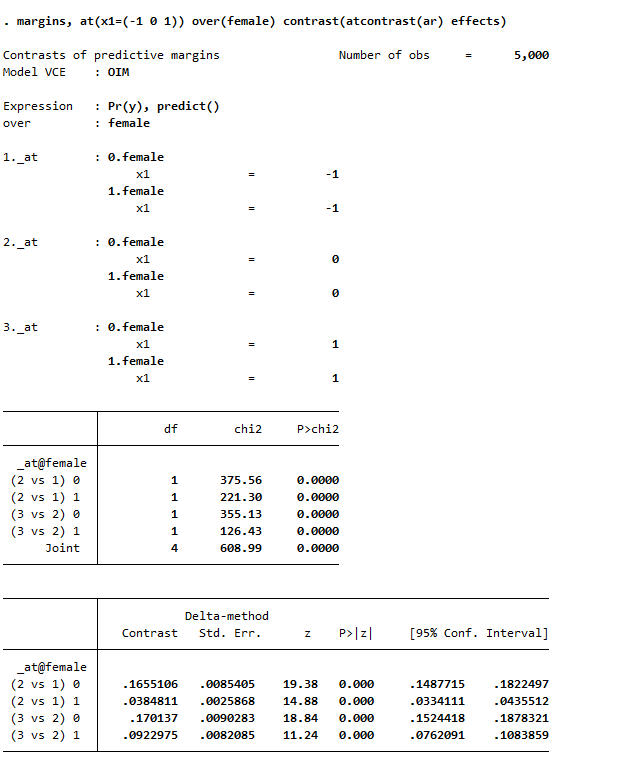
See, isn’t Stata’s margins command so nice! (For above, it actually may make more sense to use margins , at(x1=(-1 0 1)) over(female) contrast(atcontrast(ar) effects). Margins estimates the changes over the whole sample and averages filling in certain values, with over it only does the averaging within each group on over.) And finally we can test the difference in difference, to see if the discrete changes in males females from going from -1 to 0 to 1 are themselves significant:
* And can test increases of males vs females
margins r.female, at(x1=(-1(1)1)) contrast(atcontrast(ar))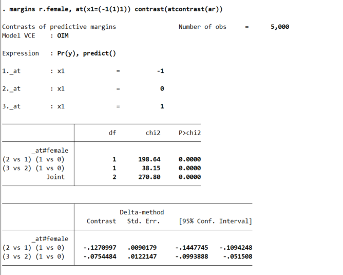
So the increase in females is 13% points smaller than the increase in males going from -1 to 0, etc.
So I have spent alot of time on the probabilities so far. I find them much easier to interpret, and I do not care so much about the fact that it doesn’t necessarily say the underlying DGP is different from males/females. But many people are interested in the odds ratios (say in case-control studies). Or generalizing to a different sample, say this is a low risk sample of females, and you want to generalize the odds ratio’s to a higher risk sample with a baseline more around 50%. Then looking at the odds ratio may make more sense.
Or so far I have not even gotten to Calli’s main point, how to test many of these effects for no differences at once. There I would just suggest the likelihood ratio test (which does not have the problems with the Wald tests on the coefficients and that the variance estimates may be off):
* Estimate restricted model
logistic y ibn.female c.x1 c.x2 c.x3, coef noconstant
estimates store restrict

* Another way to do the full interaction model
* More like separate male and female
logistic y ibn.female ibn.female#(c.x1 c.x2 c.x3), coef noconstant
estimates store full

* LRT test between models
lrtest restrict full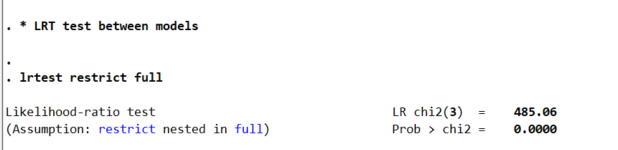
So here as expected, one rejects the null that the restricted model is a better fit to the data. But this is pretty uninformative – I rather just go to the more general model and quantify the differences.
So if you really want to look at the odds ratios, we can do that using lincom post our full interaction model:
logistic y i.female ibn.female#(c.x1 c.x2 c.x3), coef noconstant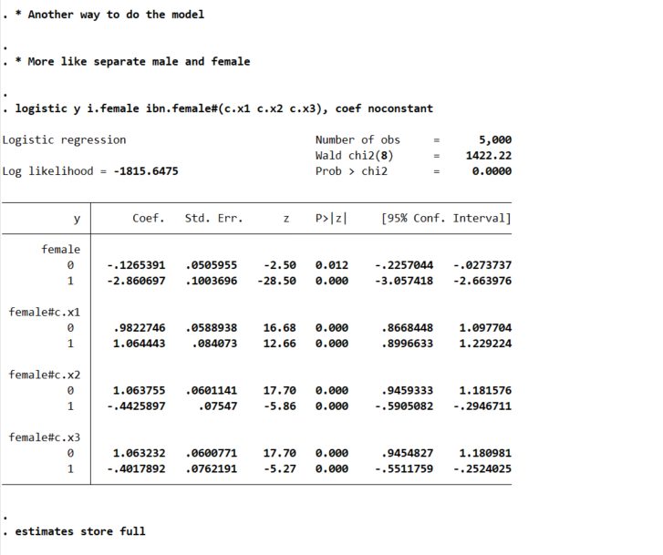
And here is an example post Wald test for equality:
lincom 0.female#c.x1 - 1.female#c.x1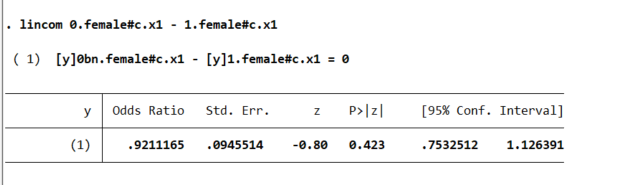
You may ask where does this odd’s ratio of 0.921 come from? Well, way back in our first full model, the interaction term for female*x1 is 0.0821688, and exp(-0.0821688) equals that odds ratio and has the same p-value as the original model I showed. And so you can see that the x1 effect is the same across each group. But estimating the other contrasts is not:
lincom 0.female#c.x2 - 1.female#c.x2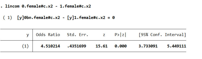
And Stata defaults this to estimating a difference in the odds ratio (as far as I can tell you can’t tell Stata to do the linear coefficient after logit, would need to change the model to glm y x, family(binomial) link(logit) to do the linear tests).
I honestly don’t know how to really interpret this – but I have been asked for it several different times by clients. Maybe they know better than me, but I think it is more to do with people just expect to be dealing with odds ratios after a logistic regression.
So we can coerce margins to give us odds ratios:
* For the odds ratios
quietly margins female, at(x3=(-1(0.1)1)) expression(exp(predict(xb)))
marginsplot , yscale(log) ylabel(0.125 0.25 0.5 1 2 4 8)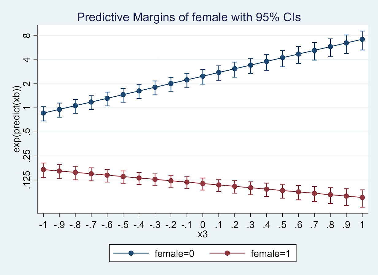
Or give us the differences in the odds ratio:
* For the contrast in the OR
quietly margins r.female, at(x3=(-1(0.1)1)) expression(exp(predict(xb)))
marginsplot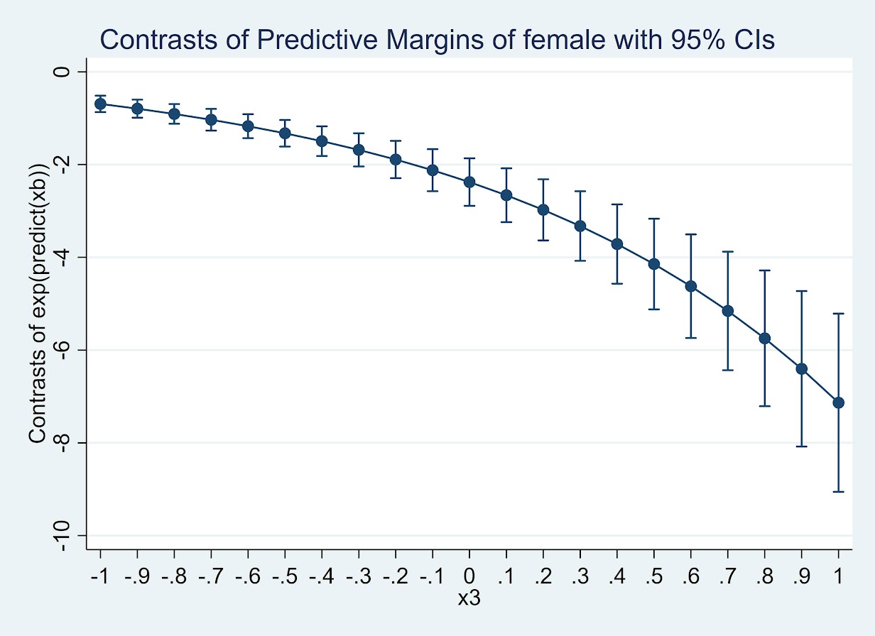
(Since it is a negative number cannot be drawn on a log scale.) But again I find it much easier to wrap my head around probabilities:
* For the probabilities
quietly margins female, at(x3=(-2(0.1)2))
marginsplot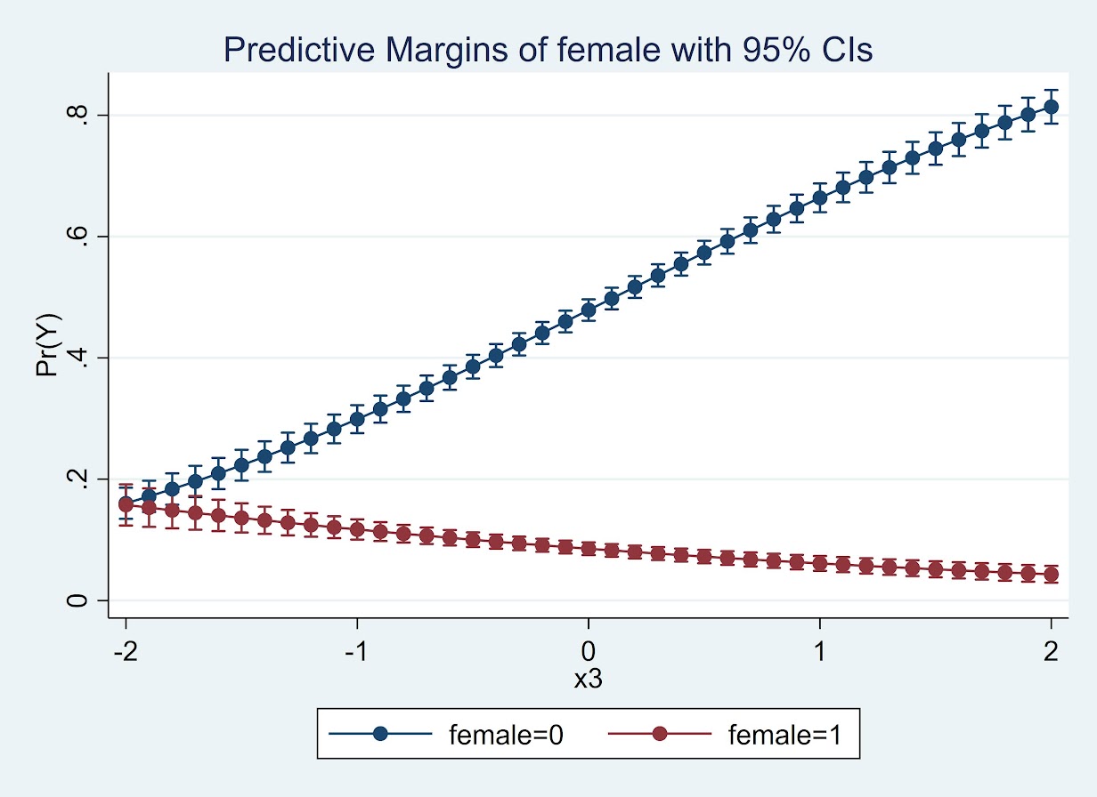
So here while x3 increases, for males it increases the probability and females it decreases. The female decrease is smaller due to the smaller baseline risk in females.
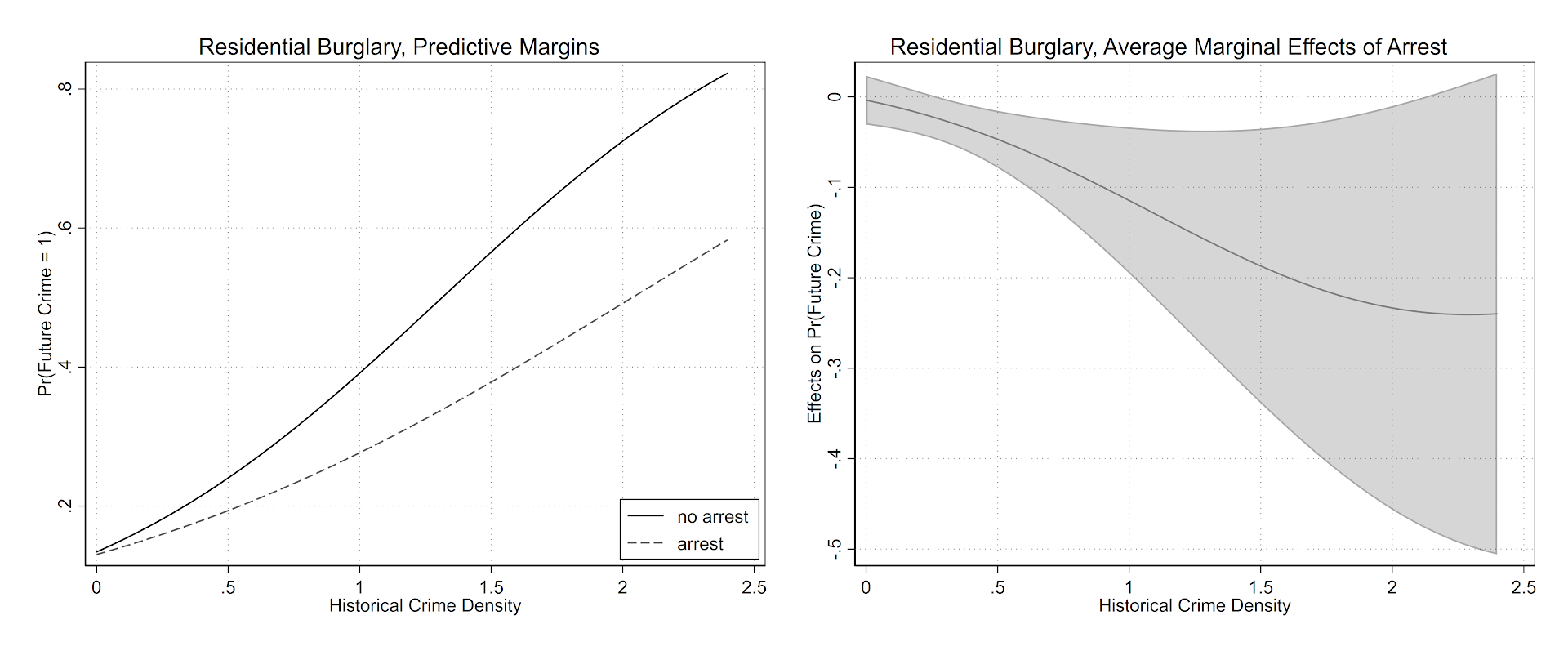
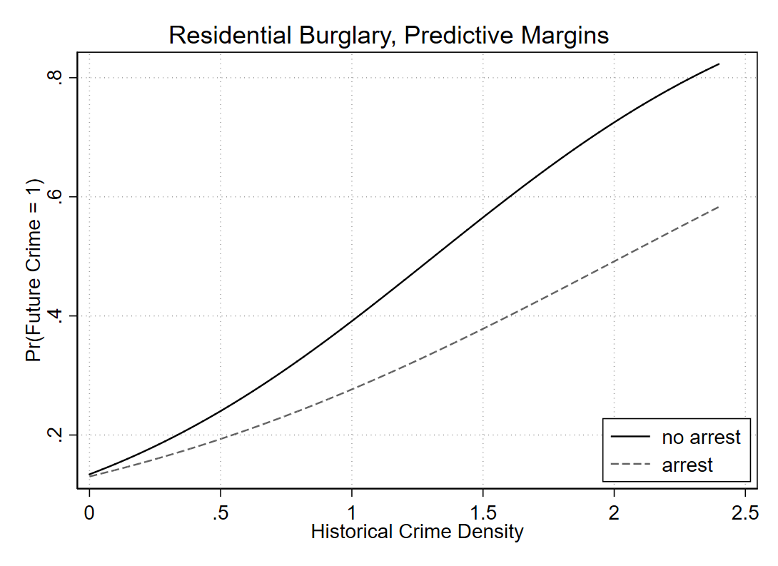
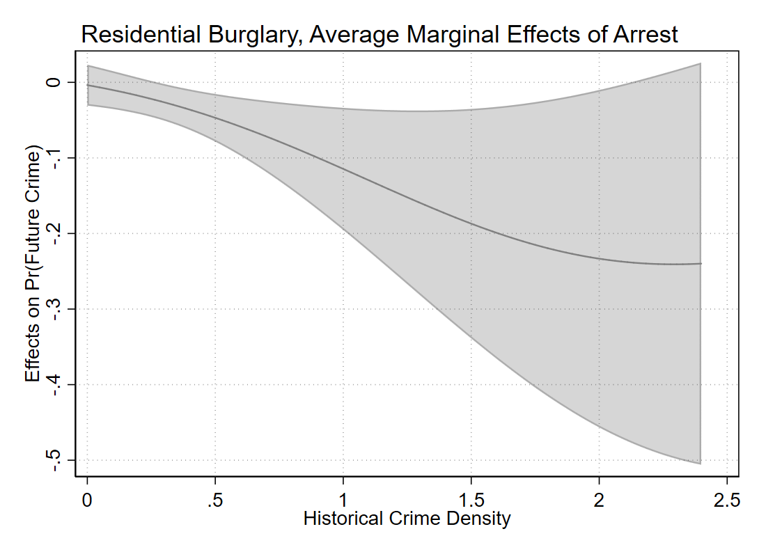
So while Calli’s original question was how to do this reasonably for many different contrasts, I would prefer the actual empirical estimates of the differences. Doing a single contrast among a small number of representative values over many variables and placing in a table/graph I think is the best way to reduce the complexity.
I just don’t find the likelihood ratio tests for all equalities that informative, and for large samples they will almost always say the more flexible model is better than the restricted model.
We estimate models to actually look at the quantitative values of those estimates, not to do rote hypothesis testing.