A changepoint logistic model in pystan

So the other day I showed how to use the mcp library in R to estimate a changepoint model with an unknown changepoint location. I was able to get a similar model to work in pystan, although it ends up being slower in practice than the mcp library (which uses JAGS under the hood). It also limits the changepoints to a specific grid of values. So offhand there isn’t a specific reason to prefer this approach to the R mcp library, but I post here to show my work. Also I illustrate that with this particular model, using 1000 simulated observations.

To be clear what this model is, instead of the many time series examples floating around about changepoints (like the one in the Stan guide), we have a model with a particular continuous independent variable x, and we are predicting the probability of something based on that x variable. It is not that different, but many of those time series examples the universe to check for changepoints is obvious, only the observed time series locations. But here we have a continuous input (distance a crime event is from a CCTV camera), but we can only check a finite number of locations. It ends up being closer in spirit to this recent post by Keith Goldfield.

So in some quick and dirty text math, here c is the changepoint location and l is the logit function:

l(Prob[y]) = intercept + b1*x; if x <= c
l(Prob[y]) = intercept + b1*x + b2*(x - c); if x > c

This model can be expanded however you want – such as other covariates that do not change with the changepoint. But for this simple simulation I am just looking at the one running variable x and the binary outcome y.

Python Code

So first, I load up the libraries I will be using, then I simulate some data. Here the changepoint is located at 0.42 for the x variable, and in the ylogit line you can see the underlying logistic regression equation.

#################################
# Libraries I am using
import pystan
import numpy as np
import pandas as pd
import statsmodels.api as sm
#################################

#################################
# Creating simulated data
np.random.seed(10)
total_cases = 1000 #30000
x = np.random.uniform(size=total_cases) #[total_cases,1]
change = 0.42
xdif = (x - change)*(x > change)
ylogit = 1.1 + -4.3*x + 2.4*xdif
yprob = 1/(1 + np.exp(-ylogit))
ybin = np.random.binomial(1,yprob)
#################################

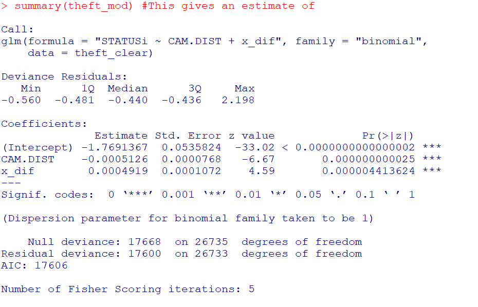
When testing out these models, one mistake I made was thinking offhand that 1,000 observations should be plenty. (Easier to run more draws with a smaller dataset.) When I had smaller effect sizes, the logistic coefficients could be pretty badly biased. So I started as a check estimating the logistic model inputting the correct changepoint location. Those biased estimates are pretty much the best case scenario you could hope for in the subsequent MCMC models. So here is an example fitting a logit model inputting the correct location for the changepoint.

#################################
#Statsmodel code to get
#The coefficient estimates 
#And standard errors for the sims
con = [1]*len(x)
xcomb = pd.DataFrame(zip(con,list(x),list(xdif)),columns=['const','x','xdif'])
log_reg = sm.Logit(ybin, xcomb).fit()
print(log_reg.summary()) 
#################################

So you can see that my coefficient estimates and the frequentist standard errors are pretty large even with 1,000 samples. So I shouldn’t expect my later MCMC model to have any smaller credible intervals than above.

So here is the Stan model. I am using pystan here, but of course it would be the same text file if you wanted to fit the model using R. (Just compiles C++ code under the hood.) Of only real note is that I show how to use the softmax function to estimate the actual mean location of the changepoint. Note that that mean summary though only makes sense if you make your grid of changepoint locations regular and fairly fine. (So if you said a changepoint could be at 0.1, 0.36, and 0.87, taking a weighted mean of those three locations doesn’t make sense.)

#################################
#Stan model
changepoint_stan = """
data {
   int<lower=1> N;
   vector[N] x;
   int<lower=0,upper=1> y[N];
   int<lower=1> Samp_Points;
   vector[Samp_Points] change;
}
transformed data {
  real log_unif;
  log_unif = -log(Samp_Points);
}
parameters {
  real intercept;
  real b_x;
  real b_c;
}
transformed parameters {
  vector[Samp_Points] lp;
  real before;
  real after;
  lp = rep_vector(log_unif, Samp_Points);
  for (c in 1:Samp_Points){
    for (n in 1:N){
      before = intercept + b_x*x[n]; 
      after = before + b_c*(x[n] - change[c]);
      lp[c] = lp[c] + bernoulli_logit_lpmf(y[n] | x[n] < change[c] ? before : after );
    }  
  }
}
model {
  intercept ~ normal(0.0, 10.0);
  b_x ~ normal(0.0, 10.0);
  b_c ~ normal(0.0, 10.0);
  target += log_sum_exp(lp);
}
generated quantities {
  vector[Samp_Points] prob_point;
  real change_loc;
  prob_point = softmax(lp);
  change_loc = sum( prob_point .* change );
}
"""
#################################

And finally I show how to prepare the data for pystan (as a dictionary), compile the model, and then draw a ton of samples. I generate a regular grid of 0.01 intervals from 0.03 to 0.97 (can’t have a changepoint outside of the x data locations, which I drew as a random uniform 0,l). Note the more typical default of 1000 tended to not converge, the effective number of samples is quite small for that many. So 5k to 10k samples in my experiments tended to converge. Note that this is not real fast either, took about 40 minutes on my machine (the Stan guesstimates for time were always pretty good ballpark figures).

#################################
# Prepping data and fitting the model

stan_dat = {'N': ybin.shape[0]}
stan_dat['change'] = np.linspace(0.03,0.97,95) #[0.1, 0.2, 0.3, 0.4, 0.5, 0.6, 0.7, 0.8, 0.9]
stan_dat['Samp_Points'] = len(stan_dat['change'])
stan_dat['x'] = x
stan_dat['y'] = ybin


sm = pystan.StanModel(model_code=changepoint_stan)
#My examples needed more like 10,000 iterations
#effective sample size very low, took about 40 minutes on my machine
fit = sm.sampling(data=stan_dat, iter=5000, 
                  warmup=500, chains=4, verbose=True)
#Prints some results at the terminal!
print(fit.stansummary(pars=['change_loc','intercept','b_x','b_c']))
#################################

So you can see the results – the credible intervals for the intercept and regression coefficient before the change point are not bad, just slightly larger than the logistic model. The credible interval for the changepoint location and the changepoint effect different are quite uncertain though. The changepoint location covers almost the whole interval I examined. It may be better to plot the individual probabilities, like Goldfield did in his post, as opposed to summarized a mean location for the distribution (which is discrete in the end based on your grid of locations you look at).

So that at least gives a partial warning that you need quite big data samples to effectively identify the changepoint location, at least for this Stan model as I have shown. I haven’t run it on my 26k actual data sample, as it will end up taking my computer around 30 hours to crunch out 10k draws with 4 chains. Next up I rather see if I can get a similar model working in pyro, as my GPU on my personal machine I think will be faster than the C++ code here. (There are probably smarter ways to vectorize the Stan model as well.)

Changepoints in CCTV Effects

So I am a big fan of using splines in regression equations to model non-linear effects. But a limitation of these is that you need to upfront say how many knots you want, as well as where the knots are. So I have explored a bit on fitting models that can identify the changepoints themselves. It was a tricky road, I tried building some in deep learning using pytorch, then tried variational auto-encoders in pyro, then pystan (marginalizing the changepoint out), and then pymc3 (using different samplers). All of my attempts failed! But when I used the R mcp library (Lindeløv, 2020), it was able to find my changepoint using simulated data. (It uses JAGS under the hood, no idea why JAGS behaved better than my other attempts.)

Usecase: Dropoff effect of CCTV on clearance rates

So in spatial criminology, a popular hypothesis is estimating distance decay effects. Ratcliffe (2012) was the first example of using a changepoint regression model to do this, showing a changepoint in the effect of bars on the spatial density of crime nearby. This has been replicated in Xu & Griffiths (2017), and in my work using machine learning and partial dependence plots I show similar changepoint patterns as well (Wheeler & Steenbeek, 2020).

One example use case though I want to mention is not in terms of estimating the spatial density of crime, but with the characteristics of the crime events themselves. Sometimes people I think mistakenly think since I have spatial data, I need to aggregate it to some areal unit, and then do analysis of that areal unit data. That approach is not per-se wrong, but is sometimes a step removed from what you want, and can result in some tricky inferences.

Take for example a recent paper looking at clearances and using RTM by Kennedy et al. (2020). What they do is spatially aggregate homicides cleared and homicides not cleared, and run RTM on each. You might be tempted to interpret if a factor is selected for both models that it does not impact clearances, but it also depends on the size of the effect. So for example, in Brooklyn for drug markets they report a rate ratio of 3.1 and 2.4 (both at the same spatial distance). To translate this into a clearance rate, you need to add the two density estimates for all cases, and then take the cleared cases as the numerator.

# Example R code
clear <- exp(-0.1 + log(3.1))
nonclear <- exp(-0.1 + log(2.4))
prop <- clear/(clear + nonclear)
prop #0.5636364

Here I am treating -0.1 as the intercept. So here this is lower, but close to the overall clearance in Brooklyn, 58%. This 56% will be the estimate iff the intercept for each equation is the same, if they are not though it could change the clearance rate estimate either way. Since the Kennedy paper did not report this, we cannot know. So for instance, if we change the intercept estimates so clearances are higher and non-clearances are lower, we get an estimate that drug markets increase clearances slightly, not decrease them:

clear <- exp(-0.05 + log(3.1))
nonclear <- exp(-0.2 + log(2.4))
prop <- clear/(clear + nonclear)
prop #0.6001124

In this example it probably won’t push them too far either way, but takes a bit of work going from the aggregate data analysis to the estimate we want, how those spatial risk factors impact the clearance rate. There is an easier way though – just incorporate your spatial features, such as the distance the nearest crime generator factor, and estimate a model on the micro level incident data. This is what Kennedy et al. (2020) do later in the paper when incorporating the RTM predictions – I just think they should have done the RTM machinery directly on this problem, instead of the two-step approach.

Examples of my work I have done this approach in the past (incorporating spatial data into the micro level incidents) is with fatalities from gun shot wounds (Circo & Wheeler, 2020). We actually investigated non-linear effects though of distance/drive-time, and did not find evidence of that. Going back to the crime clearance example though, another pre-print I examine the effects of CCTV cameras and find a diminishing effect of case clearances given the distance to the camera (Jung & Wheeler, 2019).

So here we use a pre-post design to show there are some selection effects, and we do further analysis to show this camera bump in clearances is only limited to thefts. But we set the splines at 500, 1000, and 1500 feet pre-emptively for the analysis. A reviewer critique of this is that those three locations are arbitrary (which is correct), so here I will see if I do a changepoint model that allows us to find the knot locations if it will show the same ones.

The idea behind this analysis is that CCTV are often used in investigations. Yeondae is an officer in Korea, same as here in the states first things detectives do is to go and grab CCTV footage. Analysis of cameras are often aggregated to their viewsheds, but I think estimating distance decay effects make as much sense. So events closer to the cameras presumably will provide more clear evidence than events at the border of the viewshed. A second point is that even if the event takes place off-camera, there may be evidence cross by the camera viewshed. Detectives will often try to follow individuals across multiple cameras. So both of those factors suggest a distance decay effect both within a cameras viewshed and a decaying effect even outside of the viewshed. (In addition to this, geo coordinates of crime locations are not perfectly accurate measures either, so that could cause effects outside of the viewshed as well.)

Here I am just limiting the data to the post camera data within 3000 feet for thefts, which still is over 26,000 observations. I’ve posted the data/code to follow along here.

Analysis using mcp in R

Again given my hardship in coding this up myself in python, I created a simulated data example and checked the results using mcp (which you can check in my code). Since mcp recovered my simulated changepoint, (and my python attempts did not), going to go ahead with the mcp library! First, we will import my clearance data and get rid of a few missing cases.

#################
library(mcp)
library(ggplot2)
set.seed(10)
#can see I planned on doing this in pytorch at first!
setwd('D:\\Dropbox\\Dropbox\\Documents\\BLOG\\changepoint_pytorch\\Analysis')
theft_clear <- read.csv('PostTheft_CCTV.csv')
theft_clear <- theft_clear[complete.cases(theft_clear),]
#################

So first for a reference, if I assume there is a linear changepoint at 1000 feet, here are what my results look like. Note here that this is not aggregated data to spatial locations, each row in this dataset is a theft offense, whether it was cleared, and the distance to the nearest CCTV camera.

#################
#What are the coefficients if assume a changepoint of 1000 feet
theft_clear$x_dif <- (theft_clear$CAM.DIST - 1000)*(theft_clear$CAM.DIST > 1000)
theft_mod <- glm(formula = 'STATUSi ~ CAM.DIST + x_dif', family = "binomial", data = theft_clear)
summary(theft_mod) #This gives an estimate of 
#################

And here you can visualize the results alittle easier than trying to back out probabilities for the regression equation:

#################
pred_mod <- predict(theft_mod,type='response')
plot(theft_clear$CAM.DIST,pred_mod, main="Changepoint at 1000 ft",
  xlab="Distance from Camera (ft)", ylab="Probability Clearance")
#################

So this shows clearances nearby cameras in Dallas are around 15%, and they trail off to around 9% at 1000 feet. After that they continue to tail off, but are nearly flat. But again that is assuming a change point at 1000 feet. But the mcp package lets us actual estimate the changepoint itself using Bayesian regression. Here is the set up that is equivalent to my formulation earlier, in that the changepoint cannot be discontinuous.

#################
theft_clear$x <- theft_clear$CAM.DIST 
model = list(
  STATUSi | trials(const) ~ 1 + x,
  ~ 0 + x  #joined changing rate
)

fit = mcp(model, data = theft_clear, family = binomial(), iter = 3000, adapt = 500)
#################

And then if you are following along you can go ahead and take a nap (maybe took 2 hours on my machine?), and when we get back summary(fit) gives us:

So we have very similar coefficients to the manual changepoint model earlier, but the changepoint is around 1600 feet, not 1000. (Although note these are Bayesian credible intervals, not frequentist confidence intervals.) And now to make a nice plot of the fitted model.

#Fitted values for new data
newdat <- data.frame(x = (0:300)*10)
newdat$const <- 1
newdat$CAM.DIST <- newdat$x
res <- fitted(fit, newdata = newdat)

p_pred <- ggplot(data=res) + 
  geom_line(size=1.2, color='black', aes(x = x, y = fitted)) + 
  geom_ribbon(alpha=0.5, fill='black', aes(x = x, ymin=Q2.5 , ymax=Q97.5)) + 
  scale_x_continuous(name="Feet from Camera",breaks=seq(0,3000,500),minor_breaks=NULL) + 
  scale_y_continuous(name="P(Clearance)",breaks=seq(0.06,0.16,0.02),minor_breaks=NULL) +
  theme_bw() + theme(panel.grid.major = element_line(colour = 'grey', linetype = 'dashed', size=0.1)) + 
  theme(text = element_text(size=20))

p_pred

So you can see that here it is a nearly linear drop off until 1600 feet, and then starts to climb back up. The climb up I think is likely due to selection effects, but we can’t 100% rule out displacement effects. Displacement effects could occur with cameras if detectives prioritize events around cameras and de-prioritize other events not nearby cameras. Skeptical that applies to thefts in Dallas though, as they very rarely will be assigned a detective at all.

Wrap Up

So this ended up taking me for a few different turns. One of the things I wanted to be able to test multiple changepoints, maybe if I can ever get pymc3 to give me a reasonable fit, this example is a good illustration. That should also maybe say if you should have no changepoint as well. I think maybe it is much harder to fit those models with binomial data though than with continuous (maybe good for another blog post as well, did simulations at first with 1000 observations and that was a bad idea).

One thing that would be good for evaluating whether change points are reasonable are out of sample predictive comparisons. So say estimate a no changepoint model, a linear changepoint model, and then a model with fixed spline locations. Then see which of those better fits the out of sample data. But since this is a blog post, will leave it as is. But this is a simple illustration to extend prior spatial analysis of changepoints in distance decay effects to one example – crime clearances and CCTV cameras – that I think makes alot of sense.

References