Using precision to plan experiments (SPSS)

SPSS Version 28 has some new nice power analysis facilities. Here is some example code to test the difference in proportions, with sample sizes equal between the two groups, and the groups have an underlying proportion of 0.1 and 0.2.

POWER PROPORTIONS INDEPENDENT
  /PARAMETERS TEST=NONDIRECTIONAL SIGNIFICANCE=0.05 POWER=0.6 0.7 0.8 0.9 NRATIO=1 
    PROPORTIONS=0.1 0.2 METHOD=CHISQ ESTIMATE=NORMAL CONTINUITY=TRUE POOLED=TRUE
  /PLOT TOTAL_N.

So this tells you the sample size to get a statistically significant difference (at the 0.05 level) between two groups for a proportion difference test (here just a chi square test). And you can specify the solution for different power estimates (here a grid of 0.6 to 0.9 by 0.1), as well as get a nice plot.

So this is nice for academics planning factorial experiments, but I often don’t personally plan experiments this way. I typically get sample size estimates via thinking about precision of my estimates. In particular I think to myself, I want subgroup X to have a confidence interval width of no more than 5%. Even if you want to extend this to testing the differences between groups this is OK (but will be conservative), because even if two confidence intervals overlap the two groups can still be statistically different (see this Geoff Cumming reference).

So for example a friend the other day was asking about how to sample cases for an audit, and they wanted to do subgroup analysis in errors between different racial categories. But it was paper records, so they needed to just get an estimate of the total records to sample upfront (can’t really control the subgroup sizes). I suggested to estimate the precision they wanted in the smallest subgroup of interest for the errors, and base the total sample size of the paper audit on that. This is much easier to plan than worrying about a true power analysis, in which you also need to specify the expected differences in the groups.

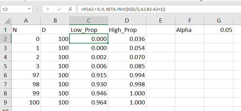
So here is a macro I made in SPSS to generate precision estimates for binomial proportions (Clopper Pearson exact intervals). See my prior blog post for different ways to generate these intervals.

* Single proportion, precision.
DEFINE !PrecisionProp (Prop = !TOKENS(1)
                      /MinN = !TOKENS(1)
                      /MaxN = !TOKENS(1)
                      /Steps = !DEFAULT(100) !TOKENS(1) 
                      /DName = !DEFAULT("Prec") !TOKENS(1) )
INPUT PROGRAM.
COMPUTE #Lmi = LN(!MinN).
COMPUTE #Step = (LN(!MaxN) - #Lmi)/!Steps.
LOOP #i = 1 TO (!Steps + 1).
  COMPUTE N = EXP(#Lmi + (#i-1)*#Step).
  COMPUTE #Suc = N*!Prop.
  COMPUTE Prop = !Prop.
  COMPUTE Low90 = IDF.BETA(0.05,#Suc,N-#Suc+1).
  COMPUTE High90 = IDF.BETA(0.95,#Suc+1,N-#Suc).
  COMPUTE Low95 = IDF.BETA(0.025,#Suc,N-#Suc+1).
  COMPUTE High95 = IDF.BETA(0.975,#Suc+1,N-#Suc).
  COMPUTE Low99 = IDF.BETA(0.005,#Suc,N-#Suc+1).
  COMPUTE High99 = IDF.BETA(0.995,#Suc+1,N-#Suc).
  END CASE.
END LOOP.
END FILE.
END INPUT PROGRAM.
DATASET NAME !DName.
FORMATS N (F10.0) Prop (F3.2).
EXECUTE.
!ENDDEFINE.

This generates a new dataset, with a baseline proportion of 50%, and shows how the exact confidence intervals change with increasing the sample size. Here is an example generating confidence intervals (90%,95%, and 99%) for sample sizes from 50 to 3000 with a baseline proportion of 50%.

!PrecisionProp Prop=0.5 MinN=50 MaxN=3000.

And we can go and look at the generated dataset. For sample size of 50 cases, the 90% CI is 38%-62%, the 95% CI is 36%-64%, and the 99% CI is 32%-68%.

For sample sizes of closer to 3000, you can then see how these confidence intervals decrease in width to changes in 4 to 5%.

But I really just generated the data this way to do a nice error bar chart to visualize:

*Precision chart.
GGRAPH
  /GRAPHDATASET NAME="graphdataset" VARIABLES=Prop N Low90 High90 Low95 High95 Low99 High99
  /GRAPHSPEC SOURCE=INLINE.
BEGIN GPL
  SOURCE: s=userSource(id("graphdataset"))
  DATA: N=col(source(s), name("N"))
  DATA: Prop=col(source(s), name("Prop"))
  DATA: Low90=col(source(s), name("Low90"))
  DATA: High90=col(source(s), name("High90"))
  DATA: Low95=col(source(s), name("Low95"))
  DATA: High95=col(source(s), name("High95"))
  DATA: Low99=col(source(s), name("Low99"))
  DATA: High99=col(source(s), name("High99"))
  DATA: N=col(source(s), name("N"))
  GUIDE: text.title(label("Base Rate 50%"))
  GUIDE: axis(dim(1), label("Sample Size"))
  GUIDE: axis(dim(2), delta(0.05))
  SCALE: linear(dim(1), min(50), max(3000))
  ELEMENT: area.difference(position(region.spread.range(N*(Low99+High99))), color.interior(color.grey), 
           transparency.interior(transparency."0.6"))
  ELEMENT: area.difference(position(region.spread.range(N*(Low95+High95))), color.interior(color.grey), 
           transparency.interior(transparency."0.6"))
  ELEMENT: area.difference(position(region.spread.range(N*(Low90+High90))), color.interior(color.grey), 
           transparency.interior(transparency."0.6"))
  ELEMENT: line(position(N*Prop))
END GPL.

So here the lightest gray area is the 99% CI, the second lightest is the 95%, and the darkest area is the 90% CI. So here you can make value trade offs, is it worth it to get an extra precision of under 10% by going from 500 samples to 1000 samples? Going from 1500 to 3000 you don’t gain as much precision as going from 500 to 1000 (diminishing returns).

It is easier to see the progression of the CI’s when plotting the sample size on a log scale (or sometimes square root), although often times costs of sampling are on the linear scale.

You can then change the macro arguments if you know your baseline is likely to not be 50%, but say here 15%:

!PrecisionProp Prop=0.15 MinN=50 MaxN=3000.

So you can see in this graph that the confidence intervals are smaller in width than the 50% – a baseline of 50% results in the largest variance estimates for binary 0/1 data, so anything close to 0% or 100% will result in smaller confidence intervals. So this means if you know you want a precision of 5%, but only have a rough guess as to the overall proportion, planning for 50% baseline is the worst case scenario.

Also note that when going away from 50%, the confidence intervals are asymmetric. The interval above 15% is larger than the interval below.

A few times at work I have had pilots that look something like “historical hit rates for these audits are 10%, I want the new machine learning model to increase that to 15%”.

So here I can say, if we can only easily use a sample of 500 cases for the new machine learning model, the precision I expect to be around 11% to 19%. So cutting a bit close to be sure it is actually above the historical baseline rate of 10%. To get a more comfortable margin we need sample sizes of 1000+ in this scenario.

Confidence intervals around proportions

So you probably learned about confidence intervals around means in your introductory statistics class. For a refresher, a confidence interval covers a particular statistic at a pre-specified rate. So if I generate 100 90% intervals around a mean, I expect that those confidence intervals would cover the true underlying mean around 90 times out of those 100. So it is a statement about the procedure overall – not any individual test.

This repeated coverage property is often not exactly what we want in statistics. But, I often find examining confidence intervals around samples to be an informative way to quantify uncertainty in estimates. For example, I have a machine learning model serving up predictions to a subsequent auditing process. I expect this to maintain a hit rate above 20%. The past week I only had a hit rate of 30/200 (15%), should I be worried? Probably not, a 95% confidence interval around that proportion is 10% to 21%.

Proportions come up so often that intro stats courses should probably talk more extensively about generating confidence intervals around them. There are many different confidence intervals for proportions, Wikipedia lists 7 different options!

I prefer where possible to use the Clopper-Pearson intervals by default. I will show an examples of generating Clopper-Pearson intervals in Excel and Python. But, another situation I have come across is I want to do these intervals entirely in SQL. For that situation, I will show how to use Agresti–Coull intervals.

Excel Clopper-Pearson

In Excel, if the A column contains the numerator, the B column contains the denominator, and if G1 has the alpha level, this brutish formula gets you the lower bound of your confidence interval;

=IF(A2=0, 0, BETA.INV($G$1/2, A2, B2-A2+1))

A here is your upper bound;

=IF(A2=B2, 1, BETA.INV(1-$G$1/2, A2+1, B2-A2))

And here is a screenshot of the filled in results:

Note for my criminology friends, you can use this for very extreme proportions as well. So say you had a homicide rate of 10 per 100,000, where the observed sample was 30 homicides in a city of 300,000. You can generate a binomial confidence interval around the proportion and then translate back to the rate per 100,000. So in that scenario, it results in a 95% confidence interval of a homicide rate of 6.7 to 14.3.

This is actually the reason I like defaulting to Clopper-Pearson. The other approximations can fail very badly for extreme tail events like this.

Python Clopper-Pearson

Here is a simple function in python to return the Clopper-Pearson intervals. This works for vectorized inputs as well (e.g. numpy arrays or pandas series).

import numpy as np
from scipy.stats import beta

def binom_int(num,den, confint=0.95):
    quant = (1 - confint)/ 2.
    low = beta.ppf(quant, num, den - num + 1)
    high = beta.ppf(1 - quant, num + 1, den - num)
    return (np.nan_to_num(low), np.where(np.isnan(high), 1, high))

And here is an example use:

hits = np.array([0, 1, 2, 3, 97, 98, 99, 100])
tries = np.array([100]*len(hits))
lowCI, highCI = binom_int(hits, tries)

Check out my prior blog post on making smoothed scatterplots on how to plot those proportion spikes in matplotlib.

SQL Agresti–Coull

So as I mentioned previously, I prefer the Clopper-Pearson intervals. This however relies on the availability of a function for the inverse beta distribution. One common situation is I just have all my tables in SQL, and I want to make a dashboard connected to a view of my tables. So the proportion of some event broken downs by days/weeks/months etc.

In that case exporting the data to python and re-uploading to the database can be a bit of a hassle, whereas creating a view is much less work. So here is an example query to calculate the proportion intervals entirely in SQL. So the initial table is a micro level table of events with 0/1 for a particular group. (This screenshot is for Access, but this should work in various databases.)

And then it is a groupby to get the original numerator, denominator, and proportion. Then a few rows calculating the adjusted proportion (add 2 to the numerator and 2*2 to the denominator), then finally this can still produce lower than 0 and higher than 1 intervals, so I cap those off.

/* This is for Access, for others may want to use SQRT() instead of SQR()
   Also may want to use CASE WHEN instead of IIF */
SELECT
   GroupID,
   SUM(Outcome) AS Num,
   COUNT(Outcome) AS Den,
   Num/Den AS Prop,
   Num + 2 AS nadj,
   Den + 2*2 as dadj,
   nadj/dadj as padj,
   2*SQR((padj/nadj)*(1 - padj)) AS zadj,
   IIF( padj < zadj, 0, padj - zadj) AS LowCI,
   IIF( (1 - padj) < zadj, 1, padj + zadj) AS HighCI
FROM ExampleData
GROUP BY GroupID;

This produces a 95% confidence interval for the final two columns. If you wanted to generate say a 99% confidence interval, you would replace the 2’s in the above table with 2.6. (In R you can do qnorm(1 - a/2), where a is 1 - confidence_level, to figure out this constant.)

What you shouldn’t use these intervals for

While I believe many applications of dashboards are well suited to including confidence intervals, confidence intervals (like p-values) are apt to be misinterpreted. One common one is that for a single 95% confidence interval, that does not mean the interval covers the true estimate with a 95% probability. This is an inference for an individual sample that is not possible in frequentist statistics – that summary would be akin to a posterior credible interval in Bayesian statistics. Confidence intervals are about the procedure, if we do this procedure over and over again, in the long run it will cover the true statistic (which we do not observe for any individual sample), according to the level we set.

Another common mistake with confidence intervals is when comparing two different intervals, them overlapping is sometimes interpreted as no difference. But this is a very conservative test (e.g. will fail to reject the null of no differences too often).

So say we were monitoring a process over time, and in October the process was 20% (40/200) and in November it was 28% (168/600). October’s confidence interval is 15% to 26%, and November’s confidence interval is 24% to 32%. So since those intervals overlap, we should conclude there are no differences correct? Not exactly, if we do a direct test for the differences in proportions (akin to a t-test of mean differences), we get a confidence interval of the difference as -14% to -1% (in R prop.test(c(40,168), c(200,600))). So in that direct hypothesis test, we would conclude October’s percent is lower than Novembers percent.

Geoff Cumming suggests that when going from individual confidence intervals to comparisons between groups, one confidence interval needs to cover the point estimate for the other group to conclude the two groups are different.

But that being said, I believe many dashboards would be improved if incorporating such confidence intervals. So although they may not always provide the test of interest, they are a good way to prevent yourself from over-interpreting noisy trends in smaller samples. In the case of comparing two intervals, for most situations I deal with, being conservative in saying this process is not showing differences is a better approach than worrying about minor fluctuations (although just depends on the use case whether that default behavior makes sense.)

So please, when reporting proportions with small samples, provide a confidence interval around those proportions!