I’m not much of a macro criminologist, but being asked questions by my dad (about Richard Rosenfeld and the Ferguson effect) and the dentist yesterday (asking about some of Trumps comments about rising crime trends) has prompted me to jump into it and give my opinion. Long story short — many sources I believe are overinterpreting short term fluctuations as more meaningful than they are.

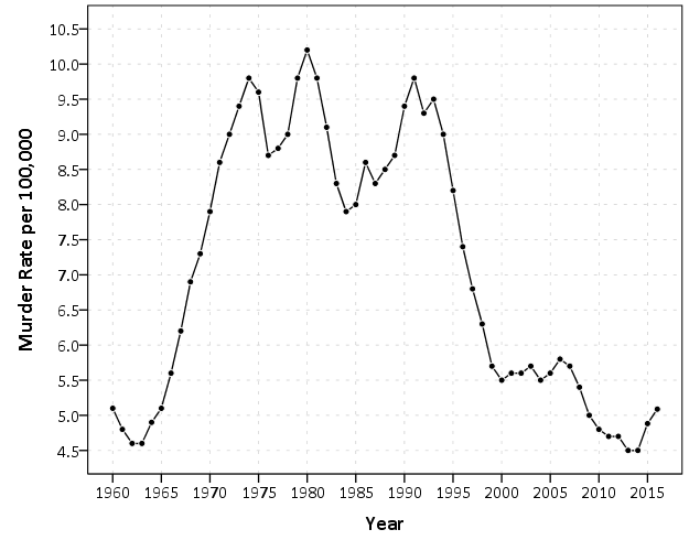
First I will tackle national crime rates. So if you have happened to walk by a TV playing CNN the past few days, you may have heard Donald Trump being criticized for his statements on crime rates. This is partially a conflation with the difference between overall levels of crime versus changes in crime over time. Basically crime is currently low compared to historical patterns, but homicide rates have been rising in the past two years. This is easier to show in a chart than to explain in words. So here is the national estimated homicide rate per 100,000 individuals since 1960.¹

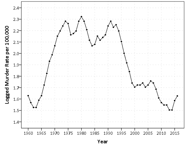
2016 is not official and is still an estimate, but basically the pattern is this – crime has been falling generally across the country since the early 1990’s. Crime rates in just the past few years have finally dropped below levels in the 1960’s, but for the past two years homicides have been increasing. So some have pointed to the increase in the past two years and have claimed the sky is falling. To say this they say the rate of change is the largest in past 40 years. There are better charts to show rates of change (a semi-log chart), but the overall look is basically the same.

You have to really squint to see that change from 2014 to 2015 is a larger jump than any of the changes over the entire period, so arguments based on the size of recent changes in the homicide rate are hyperbole (either on a linear scale or a logarithmic scale). And even if you take the recent increases over the past two years as evidence of a more general rising trend, for a broader term pattern we still have homicide rates close to a low point in the past 50 years.

For a bit of general advice — any source that gives you a percent change you always want to see the base numbers and any longer term historical trends. Any media source that cites recent increases in homicides without providing this graph of long term historical crime trends is simply misleading. I’ve seen this done in many places, see this example from the New York Times or this recent note from the Economist. So this isn’t something specific to the President.

Now, macro criminologists don’t really have any better track record explaining these patterns than macro economists have in explaining economic trends. Basically we have a bunch of patch work theories that make sense for parts of the trend, but not the entire time frame. Changes in routine activities in 1960’s, increases in incarceration, the decline of crack use, ease of calling 911 with cell-phones, lead use, abortion (just to name a few). And academics come up with new theories all the time, the most recent being the Ferguson effect — which is simply another term for de-policing.

Now a bit on trends for specific cities. How this ties in with the national trend is that some articles have been pointing out that some cities have seen increases and some have not. That is fine to point out (albeit trivial), but then the articles frequently go on generate stories about why crime is rising in those specific places. Those on the left cite civil unrest and police brutality as possible reasons (Milwaukee, St. Louis, Chicago, Baltimore), while those on the right cite the deleterious effects of police departments not being as proactive (stops in Chicago, arrests in Baltimore).

While any of these explanations may turn out reasonable in the end, I’m pretty sure most of these articles severely underappreciate the volatility in homicide rates. Take an example with St. Louis, with a city population of just over 300,000. A homicide rate of 50 individuals per 100,000 means a total of 150 murders. A homicide rate of 40 per 100,000 means 120 murders. So we are only talking about a change of 30 murders overall. Fluctuations of around 10 in the murder rate would not be unexpected for a city with a population of 300,000 individuals. The confidence interval for a rate of 150 murders per 300,000 individuals is 126 to 176 murders.²

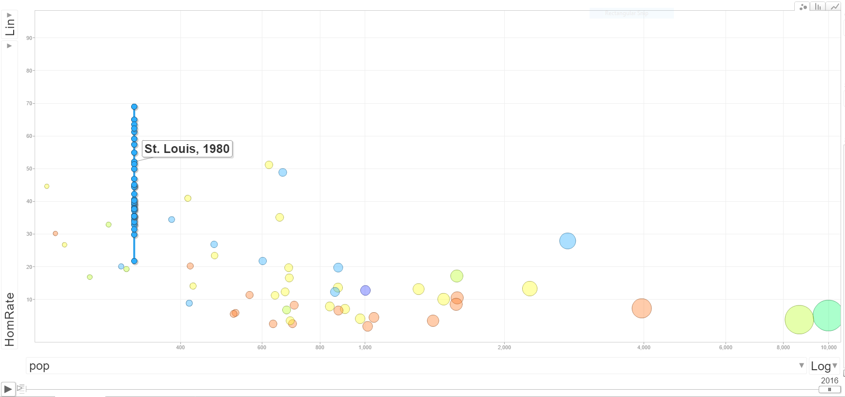
Even that though understates the typical volatility in homicide rates. As basically that assumes the proportion does not change over time. In reality crime statistics are more bursty, and show wilder fluctuations in different places.³ To show this for many cities, I use the data from the Economist article mentioned earlier, and create a motion chart of the changes in homicide rates over time. The idea behind this chart is a funnel chart. Cities with lower populations will show higher variance, and subsequently those dots on the left hand side of the chart will jump around alot more. The population figures are current and not varying, so the dots just move up and down on the Y axis.

For best viewing, make the X axis on the log scale, and size the points according to the population of the city. If you are at a desktop computer, you can open up a bigger version of the chart here.

Selecting individual points and then letting the animation run though illustrates the typical variability of crime over time. Here is the trace of St. Louis over the 36 year period.

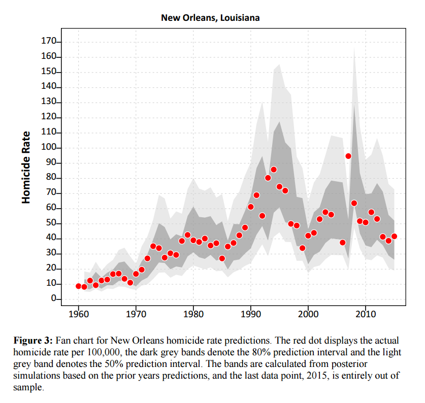
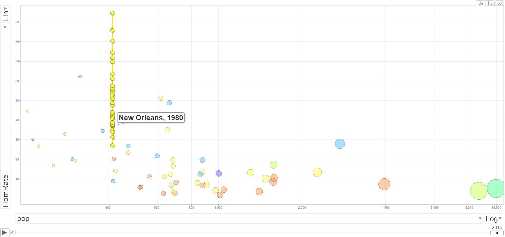
New Orleans is another good example, we have fluctuations from under 30 to over 90 in the time period.

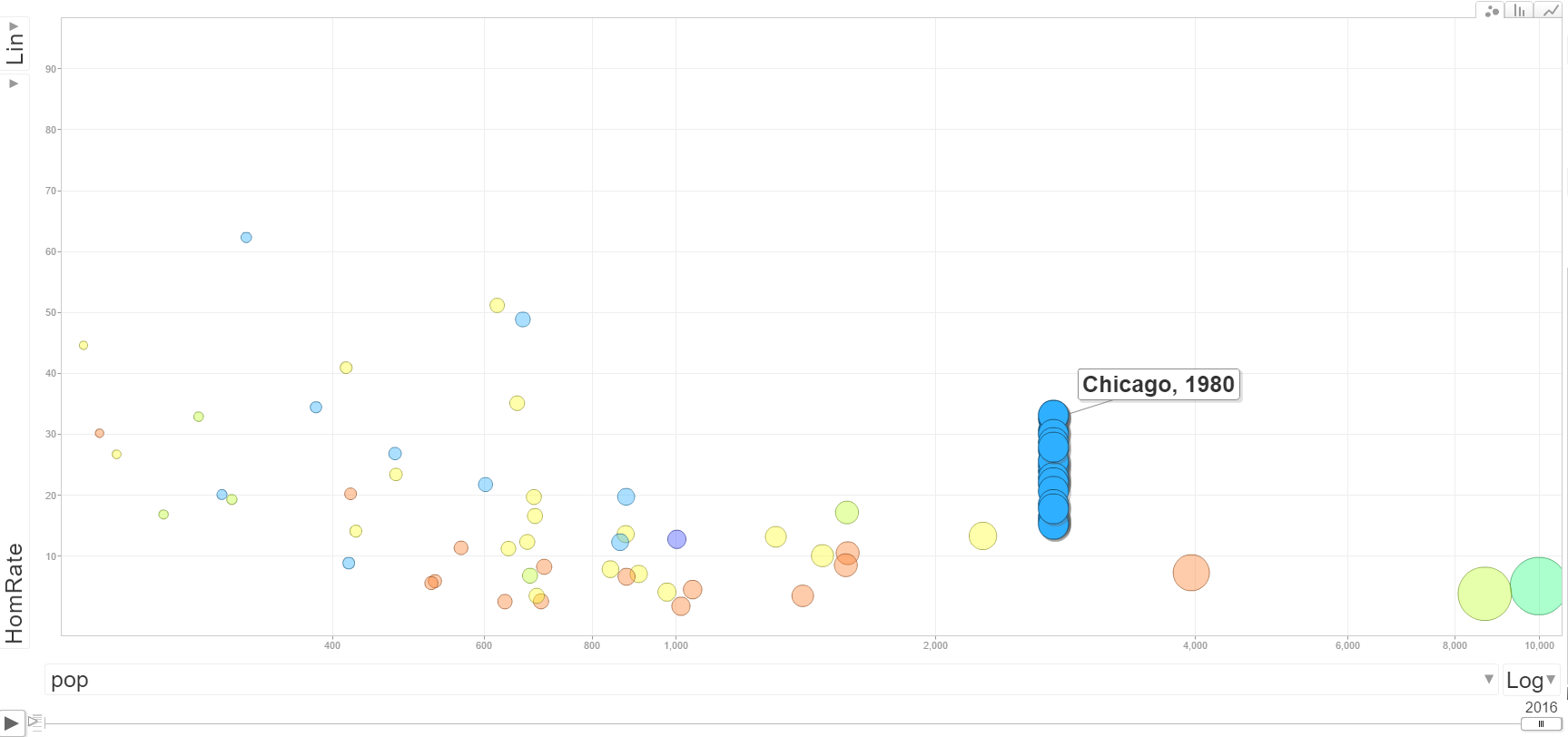
And here is Chicago, which shows less fluctuation than the smaller cities (as expected) but still has a range of homicide rates around 20 over the time period.

Howard Wainer has previously pointed this relationship out, and called it The Most Dangerous Equation. Basically, if you look you will be able to find some upward crime trends, especially in smaller cities. You need to look at it in the long term though and understand typical fluctuations to make a reasonable decision as to whether crime is increasing or if it is just typical year to year variation. The majority of news articles on the topic and just chock full of post hoc ergo propter hoc for particular cherry picked cites, and they often don’t make sense in explaining crime patterns over the past decade in those particular cities, let alone make sense for different cities experience similar conditions but not having rising homicide rates.