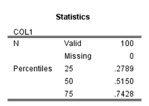
Using the New York State Online Geocoding API with Python

I’ve been very lucky doing geographic analysis in New York state, as the majority of base map layers I need, and in particular streets centerline files for geocoding, are available statewide at the NYS GIS Clearing house. I’ve written in the past how to use various Google API’s for geo data, and here I will show how one can use the NYS SAM Address database and their ESRI online geocoding service. I explored this because Google’s terms of service are restrictive, and the NYS composite locator should be more comprehensive/up to date in matches (in theory).

So first, this is basically the same as with most online API’s (at least in my limited experience), submit a particular url and get JSON in return. You just then need to parse the JSON for whatever info you need. This is meant to be used within SPSS, but the function works with just a single field address string and returns the single top hit in a list of length 3, with the unicode string address, and then the x and y coordinates. (The function is of course a valid python function, so you could use this in any environment you want.) The coordinates are specified using ESRI’s WKID (see the list for projected and geographic coordinate systems). In the code I have it fixed as WKID 4326, which is WGS 1984, and so returns the longitude and latitude for the address. When the search returns no hits, it just returns a list of [None,None,None].

*Function to use NYS geocoding API.
BEGIN PROGRAM Python.
import urllib, json

def ParsNYGeo(jBlob):
  if not jBlob['candidates']:
    data = [None,None,None]
  else:
    add = jBlob['candidates'][0]['address']
    y = jBlob['candidates'][0]['location']['y']
    x = jBlob['candidates'][0]['location']['x']
    data = [add,x,y]
  return data

def NYSGeo(Add, WKID=4326):
  base = "http://gisservices.dhses.ny.gov/arcgis/rest/services/Locators/SAM_composite/GeocodeServer/findAddressCandidates?SingleLine="
  wkid = "&maxLocations=1&outSR=4326"
  end = "&f=pjson"
  mid = Add.replace(' ','+')
  MyUrl = base + mid + wkid + end
  soup = urllib.urlopen(MyUrl)
  jsonRaw = soup.read()
  jsonData = json.loads(jsonRaw)
  MyDat = ParsNYGeo(jsonData)
  return MyDat

t1 = "100 Washington Ave, Albany, NY"
t2 = "100 Washington Ave, Poop"

Out = NYSGeo(t1)
print Out

Empt = NYSGeo(t2)
print Empt
END PROGRAM.

So you can see in the code sample that you need both the street address and the city in one field. And here is a quick example with some data in SPSS. Just the zip code doesn’t return any results. There is some funny results here though in this test run, and yes that Washington Ave. extension has caused me geocoding headaches in the past.

*Example using with SPSS data.
DATA LIST FREE / MyAdd (A100).
BEGIN DATA
"100 Washington Ave, Albany"
"100 Washinton Ave, Albany"
"100 Washington Ave, Albany, NY 12203"
"100 Washington Ave, Albany, NY, 12203"
"100 Washington Ave, Albany, NY 12206"
"100 Washington Ave, Poop"
"12222"
END DATA.
DATASET NAME NY_Add.

SPSSINC TRANS RESULT=GeoAdd lon lat TYPE=100 0 0 
  /FORMULA NYSGeo(Add=MyAdd).

LIST ALL.

New paper: Replicating Group-Based Trajectory Models of Crime at Micro-Places in Albany, NY

I posted a pre-print of a paper myself, Rob Worden and Sarah McLean have finished, Replicating Group-Based Trajectory Models of Crime at Micro-Places in Albany, NY. This is part of the work of the Finn Institute in collaboration with the Albany police department, and the goal of the project was to identify micro places (street segments and intersections) that showed long term patterns of being high crime places.

The structured abstract is below:

Objectives: Replicate two previous studies of temporal crime trends at the street block level. We replicate the general approach of group-based trajectory modelling of crimes at micro-places originally taken by Weisburd, Bushway, Lum and Yan (2004) and replicated by Curman, Andresen, and Brantingham (2014). We examine patterns in a city of a different character (Albany, NY) than those previously examined (Seattle and Vancouver) and so contribute to the generalizability of previous findings.

Methods: Crimes between 2000 through 2013 were used to identify different trajectory groups at street segments and intersections. Zero-inflated Poisson regression models are used to identify the trajectories. Pin maps, Ripley’s K and neighbor transition matrices are used to show the spatial patterning of the trajectory groups.

Results: The trajectory solution with eight classes is selected based on several model selection criteria. The trajectory of each those groups follow the overall citywide decline, and are only separated by the mean level of crime. Spatial analysis shows that higher crime trajectory groups are more likely to be nearby one another, potentially suggesting a diffusion process.

Conclusions: Our work adds additional support to that of others who have found tight coupling of crime at micro-places. We find that the clustering of trajectories identified a set of street units that disproportionately contributed to the total level of crime citywide in Albany, consistent with previous research. However, the temporal trends over time in Albany differed from those exhibited in previous work in Seattle but were consistent with patterns in Vancouver.

And here is one of the figures, a drawing of the individual trajectory groupings over the 14 year period. As always, if you have any comments on the paper feel free to shoot me an email.

ROC and Precision-Recall curves in SPSS

Recently I was tasked with evaluating a tool used to predict violence. I initially created some code to plot ROC curves in SPSS for multiple classifiers, but then discovered that the ROC command did everything I wanted. Some recommend precision-recall curves in place of ROC curves, especially when the positive class is rare. This fit my situation (a few more than 100 positive cases in a dataset of 1/2 million) and it was pretty simple to adapt the code to return the precision. I will not go into the details of the curves (I am really a neophyte at this prediction stuff), but here are a few resources I found useful:

The macro is named !Roc and it takes three parameters:

  • Class – the numeric classifier (where higher equals a greater probability of being predicted)
  • Target – the outcome you are trying to predict. Positive cases need to equal 1 and negative cases 0
  • Suf – this the the suffix on the variables returned. The procedure returns “Sens[Suf]”, “Spec[Suf]” and “Prec[Suf]” (which are the sensitivity, specificity, and precision respectively).

So here is a brief made up example using the macro to draw ROC and precision and recall curves (entire syntax including the macro can be found here). So first lets make some fake data and classifiers. Here Out is the target being predicted, and I have two classifiers, X and R. R is intentionally made to be basically random. The last two lines show an example of calling the macro.

SET SEED 10.
INPUT PROGRAM.
LOOP #i = 20 TO 70.
  COMPUTE X = #i + RV.UNIFORM(-10,10).
  COMPUTE R = RV.NORMAL(45,10).
  COMPUTE Out = RV.BERNOULLI(#i/100).
  END CASE.
END LOOP.
END FILE.
END INPUT PROGRAM.
DATASET NAME RocTest.
DATASET ACTIVATE RocTest.
EXECUTE.

!Roc Class = X Target = Out Suf = "_X".
!Roc Class = R Target = Out Suf = "_R".

Now we can make an ROC curve plot with this information. Here I use inline TRANS statements to calculate 1 minus the specificity. I also use a blending trick in GPL to make the beginning of the lines connect at (0,0) and the end at (1,1).

*Now make a plot with both classifiers on it.
GGRAPH
  /GRAPHDATASET NAME="graphdataset" VARIABLES=Spec_X Sens_X Spec_R Sens_R 
  /GRAPHSPEC SOURCE=INLINE.
BEGIN GPL
  PAGE: begin(scale(770px,600px))
  SOURCE: s=userSource(id("graphdataset"))
  DATA: Spec_X=col(source(s), name("Spec_X"))
  DATA: Sens_X=col(source(s), name("Sens_X"))
  DATA: Spec_R=col(source(s), name("Spec_R"))
  DATA: Sens_R=col(source(s), name("Sens_R"))
  TRANS: o = eval(0)
  TRANS: e = eval(1)
  TRANS: SpecM_X = eval(1 - Spec_X)
  TRANS: SpecM_R = eval(1 - Spec_R) 
  COORD: rect(dim(1,2), sameRatio())
  GUIDE: axis(dim(1), label("1 - Specificity"), delta(0.1))
  GUIDE: axis(dim(2), label("Sensitivity"), delta(0.1))
  GUIDE: text.title(label("ROC Curve"))
  SCALE: linear(dim(1), min(0), max(1))
  SCALE: linear(dim(2), min(0), max(1))
  ELEMENT: edge(position((o*o)+(e*e)), color(color.lightgrey))
  ELEMENT: line(position(smooth.step.right((o*o)+(SpecM_R*Sens_R)+(e*e))), color("R"))
  ELEMENT: line(position(smooth.step.right((o*o)+(SpecM_X*Sens_X)+(e*e))), color("X"))
  PAGE: end()
END GPL.

This just replicates the native SPSS ROC command though, and that command returns other useful information as well (such as the actual area under the curve). We can see though that my calculations of the curve are correct.

*Compare to SPSS's ROC command.
ROC R X BY Out (1)
  /PLOT CURVE(REFERENCE)
  /PRINT SE COORDINATES.

To make a precision-recall graph we need to use the path element and sort the data in a particular way. (SPSS’s line element works basically the opposite of the way we need it to produce the correct sawtooth pattern.) The blending trick does not work with this graph, but it is immaterial in interpreting the graph.

*Now make precision recall curves.
*To make these plots, need to reshape and sort correctly, so the path follows correctly.
VARSTOCASES
  /MAKE Sens FROM Sens_R Sens_X
  /MAKE Prec FROM Prec_R Prec_X
  /MAKE Spec FROM Spec_R Spec_X
  /INDEX Type.
VALUE LABELS Type
 1 'R'
 2 'X'.
SORT CASES BY Sens (A) Prec (D).
GGRAPH
  /GRAPHDATASET NAME="graphdataset" VARIABLES=Sens Prec Type
  /GRAPHSPEC SOURCE=INLINE.
BEGIN GPL
  PAGE: begin(scale(770px,600px))
  SOURCE: s=userSource(id("graphdataset"))
  DATA: Sens=col(source(s), name("Sens"))
  DATA: Prec=col(source(s), name("Prec"))
  DATA: Type=col(source(s), name("Type"), unit.category())
  COORD: rect(dim(1,2), sameRatio())
  GUIDE: axis(dim(1), label("Recall"), delta(0.1))
  GUIDE: axis(dim(2), label("Precision"), delta(0.1))
  GUIDE: text.title(label("Precision-Recall Curve"))
  SCALE: linear(dim(1), min(0), max(1))
  SCALE: linear(dim(2), min(0), max(1))
  ELEMENT: path(position(Sens*Prec), color(Type))
  PAGE: end()
END GPL.
*The sawtooth is typical.

These curves both show that X is the clear winner. In my use application the ROC curves are basically superimposed, but there is more separation in the precision-recall graph. Being very generic, most of the action in the ROC curve is at the leftmost area of the graph (with only a few positive cases), but the PR curve is better at identifying how wide you have to cast the net to find the few positive cases. In a nut-shell, you have to be willing to live with many false positives to be able to predict just the few positive cases.

I would be interested to hear other analysts perspective. Predicting violence is a popular topic in criminology, with models of varying complexity. But what I’m finding so far in this particular evaluation is basically that there are set of low hanging fruit of chronic offenders that score high no matter how much you crunch the numbers (around 60% of the people who committed serious violence in a particular year in my sample), and then a set of individuals with basically no prior history (around 20% in my sample). So basically ad-hoc scores are doing about as well predicting violence as more complicated machine learning models (even machine learning models fit on the same data).

Emailing with Python and SPSS

Emailing automated messages using Python was on my bucket list for a few projects, so here I will illustrate how to do that within SPSS. Basically the use case is if you have an automated report generated by SPSS and you want to send that automated report to certain parties (or to yourself while you are away from work). Emailing right within Python cuts out the middle annoying task of having to email yourself.

There are basically two parts of emailing within Python, 1) building the message and 2) opening your server and sending the mail. The latter is pretty simple, the former is quite tedious though. So adapting from several posts around the internet (1,2,3 plus others I don’t remember at this point), here is a function to build the email text.

*function to build message.
BEGIN PROGRAM Python.
from os.path import basename
from email.mime.multipart import MIMEMultipart
from email.mime.text import MIMEText
from email.MIMEBase import MIMEBase
from email import Encoders
from email.utils import COMMASPACE, formatdate

def make_mail(send_from, send_to, subject, text, files=None):
    assert isinstance(send_to, list)

    msg = MIMEMultipart(
        From=send_from,
        To=COMMASPACE.join(send_to),
        Date=formatdate(localtime=True),
        Subject=subject
    )
    msg.attach(MIMEText(text))

    if files != None:
      for f in files:              
        part = MIMEBase('application', 'base64')
        part.set_payload(open(f,"rb").read())
        part.add_header('Content-Disposition', 'attachment', filename=basename(f))    
        Encoders.encode_base64(part)      
        msg.attach(part)
    return msg.as_string()
END PROGRAM.

The function subsequently takes as arguments:

  • send_from: Your email address as a string
  • send_to: A list of email addresses to send to.
  • subject: A text string for the subject (please use a subject when you send an email!)
  • text: The text composition of the email in a string
  • files: A list of files with the full directory

Basically an email message is just a particular text format (which actually looking at the markup I’m slightly amazed email still functions at all). Building the markup for the to, from, subject and text in the email is tedious but relatively straightforward. However, attaching files (the main motivation for this to begin with!) is rather a pain in the butt. Here I just encode all the files in base64, and CSV, PDF, and PNG files have all worked out so far for me in my tests. (You can attach images as binary, but this approach seems to work fine at least for PNG images.)

So here is an example constructing a message, and I attach three example files. Here I just use my gmail address as both the from and to address. You can uncomment the print MyMsg at the end to see the particular markup, but it is quite long with the base64 attached files.

*Now lets make a message.
BEGIN PROGRAM Python.

us = "apwheele"
fr = us + "@gmail.com"
to = [fr]
te = "Hello!"

MyCSV = [r"C:\Users\andrew.wheeler\Dropbox\Documents\BLOG\Email_Python\Test.csv",
         r"C:\Users\andrew.wheeler\Dropbox\Documents\BLOG\Email_Python\Test.pdf",
         r"C:\Users\andrew.wheeler\Dropbox\Documents\BLOG\Email_Python\OUTPUT0.PNG"]

MyMsg = make_mail(send_from=fr,send_to=to,subject="Test",text=te,files=MyCSV)
#print MyMsg
END PROGRAM.

The second part is opening your email server and sending the message — relatively straight forward. Many people have their python functions for emailing with the username and password as part of the function. This does not make much sense to me, as they will be basically constants for a particular user, so I find it simpler to make the message and then open the server and send it. If you want to send multiple messages it makes more sense to open up the server just once. Below to make it work for yourself you just have to insert your own username and password (and possibly update the port number for your server).

*Now set up the server and send a message.
BEGIN PROGRAM Python.

us = "!!Your Username!!"
pa = "!!Your Password!!"

import smtplib
server = smtplib.SMTP('smtp.gmail.com',587)
server.starttls()

server.login(us,pa)
server.sendmail(fr,to, MyMsg)
server.quit()
END PROGRAM.

I don’t have Outlook on any of my personal machines, but hopefully it is just as simple when sending an email through a client as it is through gmail.

String substitution in Python continued

On my prior post Jon and Jignesh both made the comment that using locals() in string substitution provides for easier to read code – and is a great recommendation. What locals() does is grab the object from the local environment, so in your string if you place %(MyObject)s, and in the prior part of your code you have MyObject = "foo", it will substitute foo into the string. Using the same prior code, here is an example:

BEGIN PROGRAM Python.

var = ["V1","V2","V3"]
lab = ["Var 1","Var 2","Var 3"]

for v,l in zip(var,lab):
  spss.Submit("""
*Descriptive statistics.
FREQ %(v)s.
CORRELATIONS /VARIABLES=X1 X2 X3 %(v)s.
*Graph 1.
GRAPH /SCATTERPLOT(BIVAR)=X1 WITH %(v)s /TITLE = "%(l)s".
*Graph 2.
GRAPH /SCATTERPLOT(BIVAR)=X2 WITH %(v)s /TITLE = "%(l)s".
*Graph 3.
GRAPH /SCATTERPLOT(BIVAR)=X3 WITH %(v)s /TITLE = "%(l)s".
""" % (locals()))

END PROGRAM.

This ends up working in a similar fashion to the dictionary substitution I mentioned, just that Python makes the dictionary for you. Here is the same prior example using the dictionary with % substitution:

BEGIN PROGRAM Python.

var = ["V1","V2","V3"]
lab = ["Var 1","Var 2","Var 3"]

MyDict = {"a":v, "b":l}

for v,l in zip(var,lab):
  spss.Submit("""
*Descriptive statistics.
FREQ %(a)s.
CORRELATIONS /VARIABLES=X1 X2 X3 %(a)s.
*Graph 1.
GRAPH /SCATTERPLOT(BIVAR)=X1 WITH %(a)s /TITLE = "%(b)s".
*Graph 2.
GRAPH /SCATTERPLOT(BIVAR)=X2 WITH %(a)s /TITLE = "%(b)s".
*Graph 3.
GRAPH /SCATTERPLOT(BIVAR)=X3 WITH %(a)s /TITLE = "%(b)s".
""" % (MyDict) )

END PROGRAM.

And finally here is this example using a string template. It is basically self-explanatory.

*Using a string template.
BEGIN PROGRAM Python.
from string import Template

#Making template
c = Template("""*Descriptive statistics.
FREQ $var.
CORRELATIONS /VARIABLES=X1 X2 X3 $var.
*Graph 1.
GRAPH /SCATTERPLOT(BIVAR)=X1 WITH $var /TITLE = "$lab".
*Graph 2.
GRAPH /SCATTERPLOT(BIVAR)=X2 WITH $var /TITLE = "$lab".
*Graph 3.
GRAPH /SCATTERPLOT(BIVAR)=X3 WITH $var /TITLE = "$lab".
""")

#now looping over variables and labels
var = ["V1","V2","V3"]
lab = ["Var 1","Var 2","Var 3"]
for v,l in zip(var,lab):
  spss.Submit(c.substitute(var=v,lab=l))
END PROGRAM.

The template solution is nice because it can make the code a bit more modular (i.e. you don’t have huge code blocks within a loop). The only annoyance I can see with this is that $ does come up in SPSS code on occasion with the few system defined variables, so it needs to be escaped with a second $.

String substitution in Python

I recently had a set of SPSS syntax that iterated over multiple variables and generated many similar graphs. They were time series graphs of multiple variables, so the time stayed the same but the variable on the Y axis changed and the code also changed the titles of the graphs. Initially I was using the % string substitution with a (long) list of replacements. Here is a brief synonymous example.

*Creating some fake data.
MATRIX.
SAVE {UNIFORM(100,6)} /OUTFILE = * /VARIABLES = V1 TO V3 X1 TO X3.
END MATRIX.
DATASET NAME x.

*Crazy long string substitution.
BEGIN PROGRAM Python.
import spss

#my variable and label lists
var = ["V1","V2","V3"]
lab = ["Var 1","Var 2","Var 3"]

for v,l in zip(var,lab):
  spss.Submit("""
*Descriptive statistics.
FREQ %s.
CORRELATIONS /VARIABLES=X1 X2 X3 %s.
*Graph 1.
GRAPH /SCATTERPLOT(BIVAR)=X1 WITH %s /TITLE = "%s".
*Graph 2.
GRAPH /SCATTERPLOT(BIVAR)=X2 WITH %s /TITLE = "%s".
*Graph 3.
GRAPH /SCATTERPLOT(BIVAR)=X3 WITH %s /TITLE = "%s".
""" % (v,v,v,l,v,l,v,l))
END PROGRAM.

When you only have to substitute one or two things, "str %s and %s" % (one,two) is no big deal, but here is quite annoying having to keep track of the location of all the separate variables when the list grows. Also we are really just recycling the same object to be replaced multiple times. I thought this is python, so there must be an easier way, and sure enough there is! A simple alternative is to use the format modifier to a string object. Format can take a vector of arguments, so the prior example would be "str {0} and {1}".format(one,two). Instead of %s, you place brackets and the index position of the argument (and Python has zero based indices, so the first element is always 0).

Here is the SPSS syntax updated to use format for string substitution.

*This is much simpler using ".format" for substitution.
BEGIN PROGRAM Python.

var = ["V1","V2","V3"]
lab = ["Var 1","Var 2","Var 3"]

for v,l in zip(var,lab):
  spss.Submit("""
*Descriptive statistics.
FREQ {0}.
CORRELATIONS /VARIABLES=X1 X2 X3 {0}.
*Graph 1.
GRAPH /SCATTERPLOT(BIVAR)=X1 WITH {0} /TITLE = "{1}".
*Graph 2.
GRAPH /SCATTERPLOT(BIVAR)=X2 WITH {0} /TITLE = "{1}".
*Graph 3.
GRAPH /SCATTERPLOT(BIVAR)=X3 WITH {0} /TITLE = "{1}".
""".format(v,l))    
END PROGRAM.

Much simpler. You can use a dictionary with the % substitution to the same effect, but here the format modifier is a quite simple solution. Another option I might explore more in the future are using string templates, which seem a good candidate for long strings of SPSS code.

Dissertation Defense

The date is set, Friday, February 27, 2015 at 10:00 a.m. in Draper Hall, Room 105. As always, if you feel like sitting in the mail room and flipping through it, it is there! (My crappy picture – I do not have smart phone.)

But if not, here is a pdf copy of the dissertation. If anyone is interested, here are my hacks to get LaTex to conform to SUNY Albany’s dissertation guidelines.

The title is What we can learn from small units of analysis, and here is my abstract:

The dissertation is aimed at advancing knowledge of the correlates of crime at small geographic units of analysis. I begin by detailing what motivates examining crime at small places, and focus on how aggregation creates confounds that limit causal inference. Local and spatial effects are confounded when using aggregate units, so to the extent the researcher wishes to distinguish between these two types of effects it should guide what unit of analysis is chosen. To illustrate these differences, I examine local, spatial and contextual effects for bars, broken windows and crime using publicly available data from Washington, D.C.

Continuous color ramps in SPSS

For graphs in syntax SPSS can specify continuous color ramps. Here I will illustrate a few tricks I have found useful, as well as provide alternatives to the default rainbow color ramps SPSS uses when you don’t specify the colors yourself. First we will start with a simple set of fake data.

INPUT PROGRAM.
LOOP #i = 1 TO 30.
  LOOP #j = 1 TO 30.
    COMPUTE x = #i.
    COMPUTE y = #j.
    END CASE.
  END LOOP.
END LOOP.
END FILE.
END INPUT PROGRAM.
DATASET NAME Col.
FORMATS x y (F2.0).
EXECUTE.

The necessary GGRAPH code to make a continuous color ramp is pretty simple, just include a scale variable and map it to a color.

*Colors vary by X, bar graph default rainbow.
TEMPORARY.
SELECT IF y = 1.
GGRAPH
  /GRAPHDATASET NAME="graphdataset" VARIABLES=x y
  /GRAPHSPEC SOURCE=INLINE.
BEGIN GPL
  SOURCE: s=userSource(id("graphdataset"))
  DATA: x=col(source(s), name("x"), unit.category())
  DATA: xC=col(source(s), name("x"))
  DATA: y=col(source(s), name("y"))
  GUIDE: axis(dim(1), null())
  GUIDE: axis(dim(2), null())
  SCALE: linear(dim(2), min(0), max(1))
  ELEMENT: interval(position(x*y), shape.interior(shape.square), color.interior(xC),
           transparency.exterior(transparency."1"))
END GPL.
EXECUTE.

The TEMPORARY statement is just so the bars have only one value passed, and in the inline GPL I also specify that the outsides of the bars are fully transparent. The necessary code is simply creating a variable, here xC, that is continuous and mapping it to a color in the ELEMENT statement using color.interior(xC). Wilkinson in the Grammar of Graphics discusses that even for continuous color ramps he prefers a discrete color legend, which is the behavior in SPSS.

The default color ramp is well known to be problematic, so I will provide some alternatives. A simple choice suitable for many situations is simply a grey-scale chart. To make this you have to make a separate SCALE statement in the inline GPL, and set the aestheticMinimum and the aestheticMaximum. Besides that one additional SCALE statement, the code is the same as before.

*Better color scheme based on grey-scale.
TEMPORARY.
SELECT IF y = 1.
GGRAPH
  /GRAPHDATASET NAME="graphdataset" VARIABLES=x y
  /GRAPHSPEC SOURCE=INLINE.
BEGIN GPL
  SOURCE: s=userSource(id("graphdataset"))
  DATA: x=col(source(s), name("x"), unit.category())
  DATA: xC=col(source(s), name("x"))
  DATA: y=col(source(s), name("y"))
  GUIDE: axis(dim(1), null())
  GUIDE: axis(dim(2), null())
  SCALE: linear(dim(2), min(0), max(1))
  SCALE: linear(aesthetic(aesthetic.color.interior), 
         aestheticMinimum(color.lightgrey), aestheticMaximum(color.black))
  ELEMENT: interval(position(x*y), shape.interior(shape.square), color.interior(xC),
           transparency.exterior(transparency."1"))
END GPL.
EXECUTE.

Another option I like is to make a grey-to-red scale ramp (which is arguably diverging or continuous).

*Grey to red.
TEMPORARY.
SELECT IF y = 1.
GGRAPH
  /GRAPHDATASET NAME="graphdataset" VARIABLES=x y
  /GRAPHSPEC SOURCE=INLINE.
BEGIN GPL
  SOURCE: s=userSource(id("graphdataset"))
  DATA: x=col(source(s), name("x"), unit.category())
  DATA: xC=col(source(s), name("x"))
  DATA: y=col(source(s), name("y"))
  GUIDE: axis(dim(1), null())
  GUIDE: axis(dim(2), null())
  SCALE: linear(dim(2), min(0), max(1))
  SCALE: linear(aesthetic(aesthetic.color.interior), 
         aestheticMinimum(color.black), aestheticMaximum(color.red))
  ELEMENT: interval(position(x*y), shape.interior(shape.square), color.interior(xC),
           transparency.exterior(transparency."1"))
END GPL.
EXECUTE.

To make an nice looking interpolation with these anchors is pretty difficult, but another one I like is the green to purple. It ends up looking quite close to the associated discrete color ramp from the ColorBrewer palettes.

*Diverging color scale, purple to green.
TEMPORARY.
SELECT IF y = 1.
GGRAPH
  /GRAPHDATASET NAME="graphdataset" VARIABLES=x y
  /GRAPHSPEC SOURCE=INLINE.
BEGIN GPL
  SOURCE: s=userSource(id("graphdataset"))
  DATA: x=col(source(s), name("x"), unit.category())
  DATA: xC=col(source(s), name("x"))
  DATA: y=col(source(s), name("y"))
  GUIDE: axis(dim(1), null())
  GUIDE: axis(dim(2), null())
  SCALE: linear(dim(2), min(0), max(1))
  SCALE: linear(aesthetic(aesthetic.color.interior), 
         aestheticMinimum(color.green), aestheticMaximum(color.purple))
  ELEMENT: interval(position(x*y), shape.interior(shape.square), color.interior(xC),
           transparency.exterior(transparency."1"))
END GPL.
EXECUTE.

In cartography, whether one uses diverging or continuous ramps is typically related to the data, e.g. if the data has a natural middle point use diverging (e.g. differences with zero at the middle point). I don’t really like this advice though, as pretty much any continuous number can be reasonably turned into a diverging number (e.g. continuous rates to location quotients, splitting at the mean, residuals from a regression, whatever). So I would make the distinction like this, the ramp decides what elements you end up emphasizing. If you want to emphasize the extremes of both ends of the distribution use a diverging ramp, if you only want to emphasize one end use a continuous ramp. There are many situations with natural continuous numbers that we want to emphasize both ends of the ramp based on the questions the map or graph is intended to answer.

Going along with this, you may want the middle break to not be in the middle of the actual data. To set the anchors according to an external benchmark, you can use the min and max function within the same SCALE statement that you specify the colors. Here is an example with the black-to-red color ramp, but I set the minimum lower than the data are, so the ramp starts at a more grey location.

*Setting the break with the external min.
TEMPORARY.
SELECT IF y = 1.
GGRAPH
  /GRAPHDATASET NAME="graphdataset" VARIABLES=x y
  /GRAPHSPEC SOURCE=INLINE.
BEGIN GPL
  SOURCE: s=userSource(id("graphdataset"))
  DATA: x=col(source(s), name("x"), unit.category())
  DATA: xC=col(source(s), name("x"))
  DATA: y=col(source(s), name("y"))
  GUIDE: axis(dim(1), null())
  GUIDE: axis(dim(2), null())
  SCALE: linear(dim(2), min(0), max(1))
  SCALE: linear(aesthetic(aesthetic.color.interior), 
         aestheticMinimum(color.black), aestheticMaximum(color.red), 
         min(-10), max(30))
  ELEMENT: interval(position(x*y), shape.interior(shape.square), color.interior(xC),
           transparency.exterior(transparency."1"))
END GPL.
EXECUTE.

Another trick I like using often is to map discrete colors, and then use transparency to create a continuous ramp (most of the examples I use here could be replicated by specifying the color saturation as well). Here I use two colors and make points more towards the center of the graph more transparent. This can be extended to multiple color bins, see this post on Stackoverflow. Related are value-by-alpha maps, using more transparent to signify more uncertainty in the data (or to draw less attention to those areas). (That linked stackoverflow post wanted to emphasize the middle break for diverging data, but the point remains the same, make things you want to de-emphasize more transparent and things to want to emphasize more saturated.)

*Using transparency and fixed color bins.
RECODE x (1 THRU 15 = 1)(ELSE = 2) INTO XBin.
FORMATS XBin (F1.0).
COMPUTE Dis = -1*SQRT((x - 15)**2 + (y - 15)**2).
FORMATS Dis (F2.0).
GGRAPH
  /GRAPHDATASET NAME="graphdataset" VARIABLES=x y Dis XBin
  /GRAPHSPEC SOURCE=INLINE.
BEGIN GPL
  SOURCE: s=userSource(id("graphdataset"))
  DATA: x=col(source(s), name("x"))
  DATA: y=col(source(s), name("y"))
  DATA: Dis=col(source(s), name("Dis"))
  DATA: XBin=col(source(s), name("XBin"), unit.category())
  GUIDE: axis(dim(1), null())
  GUIDE: axis(dim(2), null())
  SCALE: cat(aesthetic(aesthetic.color.interior), map(("1",color.green),("2",color.purple)))
  ELEMENT: point(position(x*y), color.interior(XBin),
           transparency.exterior(transparency."1"), transparency.interior(Dis))
END GPL.

Another powerful visualization tool to emphasize (or de-emphasize) certain points is to map the size of an element in addition to transparency. This is a great tool to add more information to scatterplots.

*Using redundant with size.
GGRAPH
  /GRAPHDATASET NAME="graphdataset" VARIABLES=x y Dis XBin
  /GRAPHSPEC SOURCE=INLINE.
BEGIN GPL
  SOURCE: s=userSource(id("graphdataset"))
  DATA: x=col(source(s), name("x"))
  DATA: y=col(source(s), name("y"))
  DATA: Dis=col(source(s), name("Dis"))
  DATA: XBin=col(source(s), name("XBin"), unit.category())
  GUIDE: axis(dim(1), null())
  GUIDE: axis(dim(2), null())
  SCALE: linear(aesthetic(aesthetic.size), aestheticMinimum(size."1"), 
         aestheticMaximum(size."18"), reverse())
  SCALE: cat(aesthetic(aesthetic.color.interior), map(("1",color.green),("2",color.purple)))
  ELEMENT: point(position(x*y), color.interior(XBin),
           transparency.exterior(transparency."1"), transparency.interior(Dis), size(Dis))
END GPL.

Finally, if you want SPSS to omit the legend (or certain aesthetics in the legend) you have to specify a GUIDE: legend statement for every mapped aesthetic. Here is the previous scatterplot omitting all legends.

*IF you want the legend omitted.
GGRAPH
  /GRAPHDATASET NAME="graphdataset" VARIABLES=x y Dis XBin
  /GRAPHSPEC SOURCE=INLINE.
BEGIN GPL
  SOURCE: s=userSource(id("graphdataset"))
  DATA: x=col(source(s), name("x"))
  DATA: y=col(source(s), name("y"))
  DATA: Dis=col(source(s), name("Dis"))
  DATA: XBin=col(source(s), name("XBin"), unit.category())
  GUIDE: axis(dim(1), null())
  GUIDE: axis(dim(2), null())
  GUIDE: legend(aesthetic(aesthetic.color), null())
  GUIDE: legend(aesthetic(aesthetic.transparency), null())
  GUIDE: legend(aesthetic(aesthetic.size), null())
  SCALE: linear(aesthetic(aesthetic.size), aestheticMinimum(size."1"), 
         aestheticMaximum(size."18"), reverse())
  SCALE: cat(aesthetic(aesthetic.color.interior), map(("1",color.green),("2",color.purple)))
  ELEMENT: point(position(x*y), color.interior(XBin),
           transparency.exterior(transparency."1"), transparency.interior(Dis), size(Dis))
END GPL.

Some examples of using DO REPEAT in SPSS

For the majority of data management I do in SPSS, the brunt of the work is likely done in under 10 different commands. DO REPEAT is one of those commands, and I figured I would show some examples of its use.

In its simplest form, DO REPEAT simply iterates over a list of variables and can apply computations to those variables. So say in a survey you had a skip pattern, and the variables A, B, C should not be answered if someone has a value of 1 for Skip, but your current dataset just has missing data as system missing. We can use DO REPEAT to iterate over the variables and assign the missing value code.

DO REPEAT v = A B C.
  IF Skip = 1 v = 9.
END REPEAT.

Note this is not a great example, as you could simply use a DO IF Skip = 1. and nest a RECODE in that do if, but hopefully that is a clear example to start. One of the other tricks to DO REPEAT is that you can specify a counter variable to iterate over at the same time. So say you had a variable X that took integer values of 1 to 4. If you want to make dummy codes for say a regression equation, using such a counter makes short work of the process. (The VECTOR command creates the 4 original dummy variables.)

VECTOR X(4,F1.0).
DO REPEAT Xn = X1 TO X4 /#i = 1 TO 4.
  COMPUTE Xn = (X = #i).
END REPEAT.

A final trick I often find use for is to make a list of strings instead of a list of variables. For instance, say I had a list of addresses and I wanted to specifically pull out people on Main, 1st, or Central. You could do:

COMPUTE Flag = 0.
IF CHAR.INDEX(Street,"Main") > 0 Flag = 1.
IF CHAR.INDEX(Street,"1st") > 0 Flag = 2.
IF CHAR.INDEX(Street,"Central") > 0 Flag = 3.

But it is much easier to just submit your own list of strings to DO REPEAT:

COMPUTE Flag = 0.
DO REPEAT str = "Main" "1st" "Central" /#i = 1 TO 3.
  IF CHAR.INDEX(Street,str) > 0 Flag = #i.
END REPEAT.

You can similarly submit arbitrary lists of numeric values as well. With much longer lists you can see how much more expedited this code is. Anytime I find myself writing a series of very similar COMPUTE or IF statements, or chaining many variables together in one statement, I often rewrite the code to use DO REPEAT.

New paper: Tables and graphs for monitoring temporal crime patterns

I’ve uploaded a new pre-print, Tables and graphs for monitoring temporal crime patterns. The paper basically has three parts, which I will briefly recap here:

  • percent change is a bad metric
  • there are data viz. principles to constructing nicer tables
  • graphs >> tables for monitoring trends

Percent change encourages chasing the noise

It is tacitly understood that percent change when the baseline is small can fluctuate wildly – but how about when the baseline average is higher? If the average of crime was around 100 what would you guess would be a significant swing in terms of percent change? Using simulations I estimate for a 1 in 100 false positive rate you need an over 40% increase (yikes)! I’ve seen people make a big deal about much smaller changes with much smaller baseline averages.

I propose an alternative metric based on the Poisson distribution,

2*( SQRT(Post) - SQRT(Pre) )

This approximately follows a normal distribution if the data is Poisson distributed. I show with actual crime data it behaves pretty well, and using a value of 3 to flag significant values has a pretty reasonable rate of flags when monitoring weekly time series for five different crimes.

Tables are visualizations too!

Instead of recapping all the points I make in this section, I will just show an example. The top table is from an award winning statistical report by the IACA. The latter is my remake.

Graphs >> Tables

I understand tables are necessary for reporting of statistics to accounting agencies, but they are not as effective as graphs to monitor changes in time series. Here is an example, a seasonal chart of burglaries per month. The light grey lines are years from 04 through 2013. I highlight some outlier years in the chart as well. It is easy to see whether new data is an outlier compared to old data in these charts.

I have another example of monitoring weekly statistics in the paper, and with some smoothing in the chart you can easily see some interesting crime waves that you would never comprehend by looking at a single number in a table.

As always, if you have comments on the paper I am all ears.