Using LLMs to help you write is understandably a touchy subject for many. There is quite a bit of AI slop coming out now, as it is really easy to just have the LLM tools think for you and write superficially OK but ultimately garbage prose.
My recent book, LLMs for Mortals, I used Sonnet 4.1 to write the initial draft of the book (for around $5). My prior book took around a year, whereas I was able to finish this book in around two months. I definitely did a ton of copy-editing (maybe around 20-30 hours per chapter on average), but I believe around 50% of the book material is the original Sonnet generated prose.
LLMs are a tool – they can be used poorly, but I think they can be used quite well. Pangram, a tool used to detect AI writing, does not flag any of the passages in LLMs for Mortals as AI generated.

This blog post goes over my notes on how I used Claude Code to help me write (although it really is applicable to any of the current coding tools, like Codex or Gemini as well). As a meta-reference, this blog post is 100% written by myself directly, but I will link to a draft written using Claude Code later in the post for a frame of reference.
Copy Editing
First, even if you do not agree with having an LLM write for you directly, there is a use case that should be relatively uncontroversial – having an LLM take a copy-edit pass on your work.
Here is an example I used this for recently, the blog post on Crime De-Coder goes over the benefits of using an API vs local LLMs. In this conversation, you can see my original draft, and the suggestions that Claude’s desktop tool (the free version) gave.
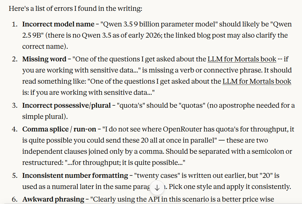
Again this is not really specific to Claude (this would have worked fine in ChatGPT as well). LLMs are good for not only spelling errors, but grammatical issues that spell check will not catch, as well as just more general copy-editing advice on the content.
One point of this – to replicate my setup, you need to write in plain text. Most of the things I write are in some form of markdown (plain markdown for blog posts, and Quarto for longer reports/books/etc). This makes it much easier to use the tools, especially the command line interface (CLI) tools like Claude Code.
Writing New Content
There are two big issues currently with LLM writing:
- it is potentially wrong
- current LLM writing has a particular style that is itself becoming noticeable
The first bullet, you need to review what it writes. It is much easier to have it write on content you are an expert in, so it is easier to review and spot errors. (It is the same current problem with using the tools to help you write computer code – they are boons for seniors but can write a ton of slop that more neophyte coders have a hard time spotting issues.)
The second bullet, having the style mimic your own, is what I am going to discuss here. It is worth understanding at a high level how generative AI LLMs work – if you ask “answer question X” vs “here is a book, …., answer question X” the LLM will generate a different response. The first part in the former prompt, “here is a book, …” is what is referred to the context. Current models have context windows (how large of a potential input) at around 500,000 words (technically they are around 1 million tokens, one word is often multiple tokens though).
You generally do not want to fill up the context window 100%, but 500,000 words is a very large number – just including text it would be multiple books. Another common prompting technique is what is called k-shot examples. It will typically go like
example input1: ...text... expected_output: ...blah...
example input2: ...diff text... expected_output: ...blah2...
....
This is what you place in the context window, then submit your usual prompt, and have the LLM generate the content. It is giving prior examples to help guide the LLM what you expect the final output to look like. This works the same way with writing – give the LLM prior examples of your writing to help it mimic your future style.
To keep it simple, I have created an example on github to follow along. Basically just have your prior writing (in text!), and then ask Claude Code something like:
review my prior blog posts in folder /blogposts, I am going to have you write a new blog post on topic X given the outline *after* you review the textThen after your prior work is in the context window, feed the LLM an outline for what you want to write. In this example, I put the outline in an actual text file and said:
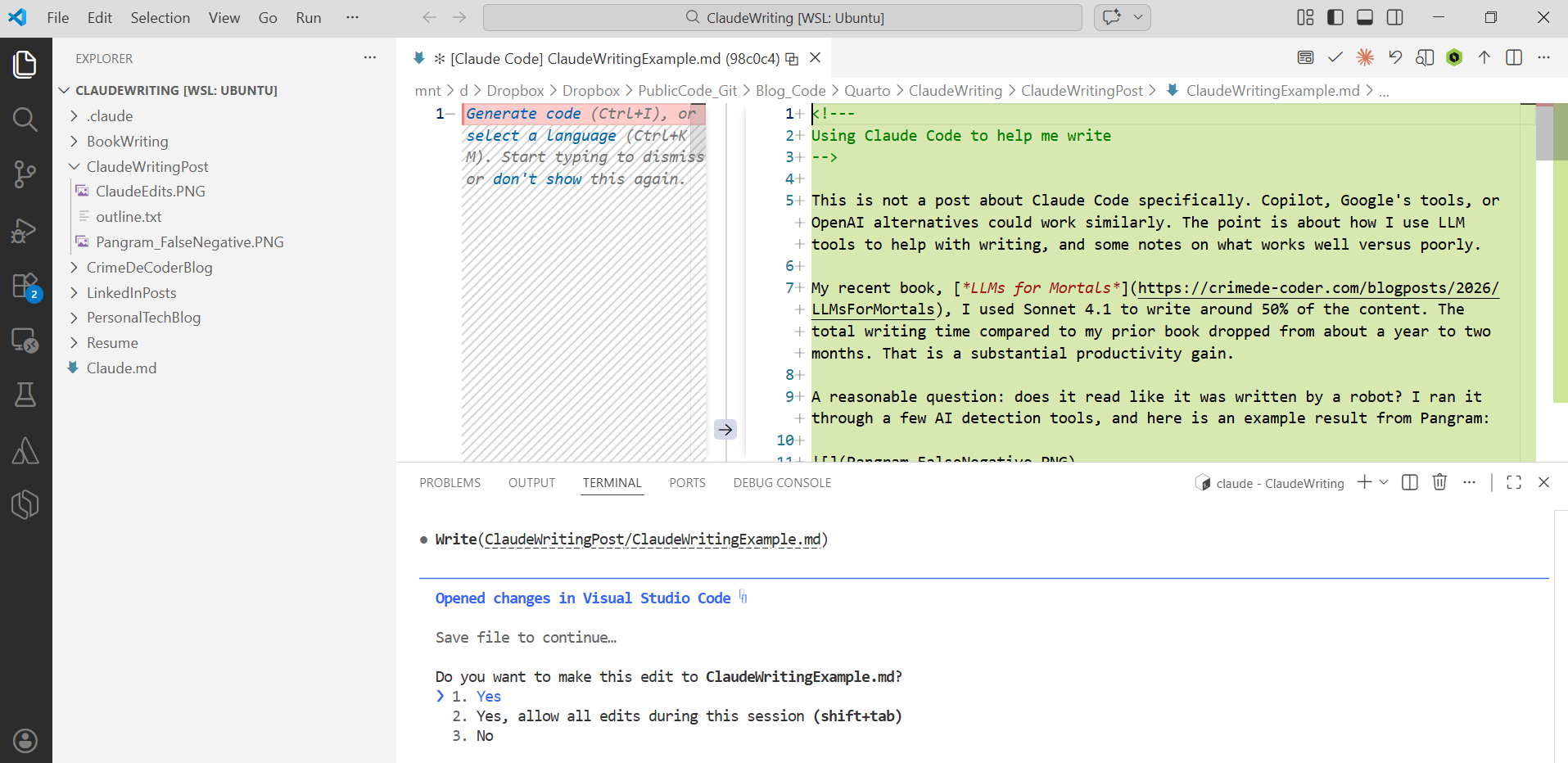
In the ClaudeWritingPost folder, review the outline.txt, then create a new md
file, called ClaudeWritingExample.md, filling in the sections based on the
outline
Claude Code will then go and review the text file with the outline and write the post. In the github repo I have my original outline for this same post, so you can see side-by-side.
You can technically write custom commands and skills with Claude Code (or the other CLI tools) to save the steps of typing two prompts, but to keep it simple for folks I am just showing the two steps manually. It is really just those two steps – get your prior examples into the context window, and then feed an outline for what else to write.
In the Github repo you can see some additional Claude.md files – these are files that include additional instructions. A common one I say is “do not include emojis”. LLM writing also tends to be verbose and have excessive lists. So I have instructions to avoid those as well.
The written blog post is not bad – I would suggest to go and read it as a proof of concept (I exported the session, can see it cost around fifty cents). Part of the reason I do not typically worry about blog posts is that I often add in things/change things in the process of writing. So you can see my personally written post is longer and has a few more elements.
So when would you use it? Technical writing, like writing tutorials in python, it works very well. Hence I could have it write the first pass on my LLM book and keep 50% of the content. I may use it for blog posts in the future (if I felt compelled to write something every day). But will not take that plunge for now.
For longer pieces, like an entire paper or a book, I suggest to not only make a detailed outline, but to also have the LLM write it in smaller sections. This both helps with reviewing the content, as well as to keep the LLM on track if you make edits/changes as you go. (Longer conversations it is more likely to degrade and make repeated errors.)
An Extra Note About Citations
I am not writing academic papers much anymore, but another fundamental problem with LLM writing is hallucinating citations. If you write in text markdown files, my suggestion is fairly simple – have the papers you want to cite in a bibtex file, and in-line in markdown, only cite papers in the form:
Citation, @item1 says blah [@item1; @item2]. For a specific page quote [@item1 p. 34-35].The way I write my outlines, it typically is like write a paragraph about X, cite papers a,b,c. So my personal style of progressively filling in an outline works well with LLMs.
So this presumes you already have a list of papers (and are not using the LLM to dynamically write your lit review based on papers you have not read). Next time I actually need to write an academic paper, I may write up an MCP tool to query Semantic Scholar’s API and create a nice bibtex file.
But the solution here is again you need to review the output for accuracy. People without these tools are lazy and cite things they have not read already, so that will continue to happen (the tools just make it easier). Those that figure out how to use the tools appropriately though can be much more productive writing.