AMA: Advice on clustering

Ashely Evan’s writes in with a question:

I very recently started looking into clustering which I’ve only touched upon briefly in the past.

I have an unusual dataset, with dichotomous or binary responses for around 25000 patents and 35 categories.

Would you be able to recommend a suitable method, I couldn’t see if you’d done anything like this before on your site.

It’s a similar situation to a survey with 25000 respondents and 35 questions which can only be answered yes/no (1 or 0 is how I’ve represented this in my data).

The motivation for clustering would be to identify which questions/areas naturally cluster together to create distinct profiles and contrast differences.

I tried the k modes algorithm in r, using an elbow method which identified 3 clusters. This is a decent starting point, the size of the clusters are quite unbalanced, two had one common category for every result and the other category was quite fragmented.

I figured this topic would be a good one for the blog. The way clustering is treated in many data analysis courses is very superficial, so this contains a few of my thoughts to help people in conducting real world cluster analysis.

I have never done any project with similar data. So caveat emptor on advice!

So first, clustering can be tricky, since it is very exploratory. If you can put more clear articulation what the end goal is, I always find that easier. Clustering will always spit out solutions, but having clear end-goals makes it easier to tell whether the clustering has any face validity to accomplish those tasks. (And sometimes people don’t want clustering, they want supervised learning or anomaly detection.) What is the point of the profiles? Do you have outcomes you expect with them (like people do in market segmentation)?

The clustering I have done is geospatial – I like a technique called DBSCAN – this is very different than K-means (which every point is assigned into a cluster). You just identify areas of many cases nearby in space, and if this area has greater than some threshold, it is a local cluster. K-means being uneven is typical, as every point needs to be in a cluster. You tend to have a bunch of junk points in the cluster (so sometimes focusing on the mean or modal point in k-means may be better than looking at the whole distribution).

I don’t know if DBSCAN makes sense though for 0/1 data. Another problem with clustering many variables is what is called the curse of dimensionality. If you have 3 variables, you can imagine drawing your 3d scatterplot and clustering of those points in that 3d space. You cannot physically imagine it, but clustering with more variables is like this visualization, but in many higher dimensions.

What happens though is that in higher dimensions, all of the points get pushed away from each other, and closer to the hull of the that k-dimensional sphere (or I should say box here with 0/1 data). So the points tend to be equally far apart, and so clusters are not well defined. This is a different problem, but I like this example of averaging different dimensions to make a pilot that does not exist, it is the same issue.

There may be ways to take your 35 inputs and reduce down to fewer variables (the curse of dimensionality comes at you fast – binary variables may not be as problematic as continuous ones, but it is a big deal for even as few as 6-10 dimensions).

So random things to look into:

  • factor analysis of dichotomous variables (such as ordination analysis), or simply doing PCA on the columns may identify redundant columns (this doesn’t get you row wise clusters, but PCA followed by K-means is a common thing people do). Note that this only applies to independent categories, turning a single category into 35 dummy variables and then doing PCA does not make sense.

  • depending on what you want, looking at association rules/frequent item sets may be of interest. So that is identifying cases that tend to cluster with pairs of attributes.

  • for just looking at means of different profiles, latent class analysis I think is the “best” approach out of the box (better than k-means). But it comes with its own problems of selecting the number of groups.

The regression + mixture model I think is a better way to view clustering in a wider variety of scenarios, such as customer segmentation. I really do not like k-means, I think it is a bad default for many real world scenarios. But that is what most often gets taught in data science courses.

The big thing is though you need to be really clear about what the goals of the analysis are – those give you ways to evaluate the clustering solutions (even if those criteria are only fuzzy).

Trajectories are not real

I recently published my peer review of Andresen, Curman, and Linning (2016), The Trajectories of Crime at Places: Understanding the Patterns of Disaggregated Crime Types. In it I probably come off as a bit curmudgeonly, but in my defense I voted for revise-and-resubmit (I don’t know why Publons does not have a field to note this in your review).

I’ve gotten a few questions about doing trajectory analysis, so I figured I would come out and make my opinion pretty clear — I don’t think such trajectories exist. Part of the motivation in my paper to estimate the trajectories in Albany was to replicate Weisburd’s work in Seattle. (Andresen et al. (2016) give the same reasoning for their currently cited article — at least to stick with the k-means clustering procedure anyway.) But that does not mean I think distinct groups of trajectories exist. I tried to sneak this in wherever possible in my JQC article, but if you just quickly skimmed it you might not have that impression.

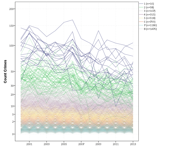
For an ugly image I generated but did not make the paper, here is my reasoning that discrete trajectories do not exist:

Superimposed_Chart

You can see that each individual grouping (unique colors) basically overlaps with each other. This solution passes all the usual model based criteria for trajectory groups, and each individual line tends to have a very high posterior probability of assignment to its respective group. Despite this there is essentially no separation between the groups – they all just blend into one another. If people plotted the individual trajectories this would be more obvious in other work, but people almost always solely plot the predicted trajectories.

Now, although I’m pretty sure that the clusters are not real (at least in the data I have seen) that does not mean that I don’t think they can be useful. Longitudinal data can be complicated, and clustering trajectories are a simple procedure to make sense of it. For a good example of its utility, Weisburd et al., (2015) used it to assign blocks for a randomized experiment. This is a slightly more robust way than ranking based some prior time interval (in that it might out some weird trajectory groups that simple averaging would not).

I believe it is similar in utility to creating hot spot polygons or maps of kernel density estimates. They can illuminate the patterns the messy data, but the hot spot the computer spits out is not a real entity – it is something we arbitrarily created.

Estimating group based trajectory models using SPSS and R

For a project I have been estimating group based trajectory models for counts of crime at micro places. Synonymous with the trajectory models David Weisburd and colleagues estimated for street segments in Seattle. Here I will show how using SPSS and the R package crimCV one can estimate similar group based trajectory models. Here is the crimCV package help and here is a working paper by the authors on the methodology. The package specifically estimates a zero inflated poisson model with the options to make the 0-1 part and/or the count part have quadratic or cubic terms – and of course allows you specify the number of mixture groups to search for.

So first lets make a small set of fake data to work with. I will make 100 observations with 5 time points. The trajectories are three separate groups (with no zero inflation).

*Make Fake data.
SET SEED 10.
INPUT PROGRAM.
LOOP Id = 1 TO 100.
END CASE.
END LOOP.
END FILE.
END INPUT PROGRAM.
DATASET NAME OrigData.
*Make 3 fake trajectory profiles.
VECTOR Count(5,F3.0).
DO REPEAT Count = Count1 TO Count5 /#iter = 1 TO 5.
COMPUTE #i = #iter - 3.
COMPUTE #ii  = #i**2.
COMPUTE #iii = #i**3.
  DO IF Id <= 30.
    COMPUTE #P    = 10 + #i*0.3 + #ii*-0.1 + #iii*0.05.
    COMPUTE Count = RV.POISSON(#P).
  ELSE IF Id <=60.
    COMPUTE #P    =  5 + #i*-0.8 + #ii*0.3 + #iii*0.05.
    COMPUTE Count = RV.POISSON(#P).
  ELSE. 
    COMPUTE #P    =  4 + #i*0.8 + #ii*-0.5 + #iii*0.
    COMPUTE Count = RV.POISSON(#P).
  END IF.
END REPEAT.
FORMATS Id Count1 TO Count5 (F3.0).
EXECUTE.

Note The crimCV package wants the data to be wide format for the models, that is each separate time point in its own column. Now we can call R code using BEGIN PROGRAM R to recreate the wide SPSS dataset in an R data frame.

*Recreate SPSS data in R data frame.
BEGIN PROGRAM R.
casedata <- spssdata.GetDataFromSPSS(variables=c("Id","Count1","Count2",
                                                "Count3","Count4","Count5")) #grab data from SPSS
casedataMat <- as.matrix(casedata[,2:6]) #turn into matrix
#summary(casedata) #check contents
#casedataMat[1:10,1:5]
END PROGRAM.

Now to fit one model with 3 groups (without calculating the cross validation statistics) the code would be as simple as:

*Example estimating model with 3 groups and no CV.
BEGIN PROGRAM R.
library(crimCV)
crimCV(casedataMat,3,rcv=FALSE,dpolyp=3,dpolyl=3)
END PROGRAM.

But when we are estimating these group based trajectory models we don’t know the number of groups in advance. So typically one progressively fits more groups and then uses model selection criteria to pick the mixture solution that best fits the data. Here is a loop I created to successively estimate models with more groups and stuffs the models results in a list. It also makes a separate data frame that saves the model fit statistics, so you can see which solution fits the best (at least based on these statistics). Here I loop through estimates of 1 through 4 groups (this takes about 2 minutes in this example). Be warned – here are some bad programming practices in R (the for loops are defensible, but growing the lists within the loop is not – they are small though in my application and I am lazy).

*looping through models 1 through 4.
BEGIN PROGRAM R.
results <- c()  #initializing a set of empty lists to store the seperate models
measures <- data.frame(cbind(groups=c(),llike=c(),AIC=c(),BIC=c(),CVE=c())) #nicer dataframe to check out model 
                                                                            #model selection diagnostics
max <- 4 #this is the number of grouping solutions to check

#looping through models
for (i in 1:max){
    model <- crimCV(casedataMat,i,rcv=TRUE,dpolyp=3,dpolyl=3)
    results <- c(results, list(model))
    measures <- rbind(measures,data.frame(cbind(groups=i,llike=model$llike,
                                          AIC=model$AIC,BIC=model$BIC,CVE=model$cv)))
    #save(measures,results,file=paste0("Traj",as.character(i),".RData")) #save result
    }
#table of the model results
measures
END PROGRAM.

In my actual application the groups take a long time to estimate, so I have the commented line saving the resulting list in a file. Also if the model does not converge it breaks the loop. So here we see that the mixture with 3 groups is the best fit according to the CVE error, but the 2 group solution would be chosen by AIC or BIC criteria. Just for this tutorial I will stick with the 3 group solution. We can plot the predicted trajectories right within R by selecting the nested list.

*plot best fitting model.
BEGIN PROGRAM R.
plot(results[[3]])
#getAnywhere(plot.dmZIPt) #this is the underlying code
END PROGRAM.

Now the particular object that stores the probabilities is within the gwt attribute, so we can transform this to a data frame, merge in the unique identifier, and then use the STATS GET R command to grab the resulting R data frame back into an SPSS dataset.

*Grab probabiltiies back SPSS dataset.
BEGIN PROGRAM R.
myModel <- results[[3]] #grab model
myDF <- data.frame(myModel$gwt) #probabilites into dataframe
myDF$Id <- casedata$Id #add in Id
END PROGRAM.
*back into SPSS dataset.
STATS GET R FILE=* /GET DATAFRAME=myDF DATASET=TrajProb.

Then we can merge this R data frame into SPSS. After that, we can classify the observations into groups based on the maximum posterior probability of belonging to a particular group.

*Merge into original dataset, and the assign groups.
DATASET ACTIVATE OrigData.
MATCH FILES FILE = *
  /FILE = 'TrajProb'
  /BY ID
  /DROP row.names.
DATASET CLOSE TrajProb.
*Assign group based on highest prob.
*If tied last group wins.
VECTOR X = X1 TO X3.
COMPUTE #MaxProb = MAX(X1 TO X3).
LOOP #i = 1 TO 3.
  IF X(#i) = #MaxProb Group = #i.
END LOOP.
FORMATS Group (F1.0).

Part of the motivation for doing this is not only to replicate some of the work of Weisburd and company, but that it has utility for identifying long term hot spots. Part of what Weisburd (and similarly I am) finding is that crime at small places is pretty stable over long periods of time. So we don’t need to make up to date hotspots to allocate police resources, but are probably better off looking at crime over much longer periods to identify places for targeted strategies. Trajectory models are a great tool to help identify those long term high crime places, same as geographic clustering is a great tool to help identify crime hot spots.