Hyperparameter tuning for Random Forests

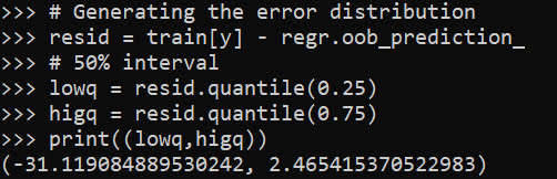
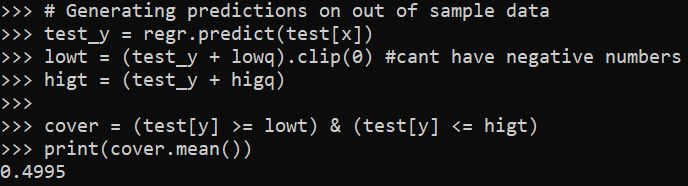
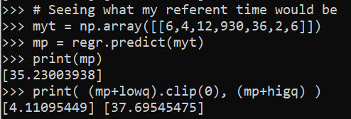
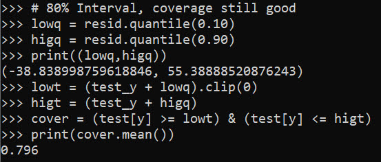
Motivated to write this post based on a few different examples at work. One, we have periodically tried different auto machine learning (automl) libraries at work (with quite mediocre success). They are OK for a baseline, not so much for production. Two, a fellow data scientist was trying some simple hyperparameter search in random forests, and was searching over all the wrong things.

For those not familiar, automl libraries, such as data robot or databricks automl, typically do a grid search over different models given a particular problem (e.g. random forest, logistic regression, XGBoost, etc.). And within this you can have variants of similar models, e.g. RFMod1(max-depth=5) vs RFMod2(max-depth=10). Then given a train/test split, see which model wins in the test set, and then suggests promoting that model into production.

My experience at work with these different libraries (mostly tabular medical records data), they choose XGBoost variants at a very high frequency. I think this is partially due to poor defaults for the hyperparameter search in several of these automl libraries. Here I will just be focused on random forests, and to follow along I have code posted on Github.

Here I am using the NIJ recidivism challenge data I have written about in the past, and for just some upfront work I am loading in various libraries/functions (I have the recid functions in the githup repo). And then making it easy to just load in the train/test data (with some smart feature engineering already completed).

from datetime import datetime
import matplotlib.pyplot as plt
import numpy as np
import optuna
import pandas as pd
from sklearn.metrics import brier_score_loss, roc_auc_score
from sklearn.model_selection import train_test_split
from sklearn.ensemble import RandomForestClassifier
import recid # my custom NIJ recid funcs

# Read in data and feature engineering
train, test = recid.fe()

Now first, in terms of hyperparameter tuning you need to understand the nature of the model you are fitting, and how those hyperparameters interact with the model. In terms of random forests for example, I see several automl libraries (and my colleague) doing a search over the number of trees (or estimators in sklearn parlance). Random forests the trees are independent, and so having more trees is always better. It is sort of like saying would you rather me do 100 simulations or 1,000,000 simulations to estimate a parameter – the 1,000,000 will of course have a more accurate estimate (although may be wasteful, as the extra precision is not needed).

So here, using the NIJ defined train/test split, and a set of different fixed parameters (close to what I typically default to for random forests). I show how AUC or the Brier Score changes with the number of trees, over a grid from 10 to 1000 trees:

# Loop over tree sizes
ntrees = np.arange(10,1010,10)
auc, bs = [], []

# This is showing number of estimators is asymptotic
# should approach best value with higher numbers
# but has some variance in out of sample test
for n in ntrees:
    print(f'Fitting Model for ntrees:{n} @ {datetime.now()}')
    # Baseline model
    mod = RandomForestClassifier(n_estimators=n, max_depth=5, min_samples_split=50)
    # Fit Model
    mod.fit(train[recid.xvars], train[recid.y1])
    # Evaluate AUC/BrierScore out of sample
    pred_out = mod.predict_proba(test[recid.xvars])[:,1]
    auc.append(roc_auc_score(test[recid.y1], pred_out))
    bs.append(brier_score_loss(test[recid.y1], pred_out))

# Making a plot of the 
fig, (ax1, ax2) = plt.subplots(2, figsize=(6,8))
ax1.plot(ntrees, auc)
ax1.set_title('AUC')
ax2.plot(ntrees, bs)
ax2.set_title('Brier Score')
plt.savefig('Ntree_grid.png', dpi=500, bbox_inches='tight')

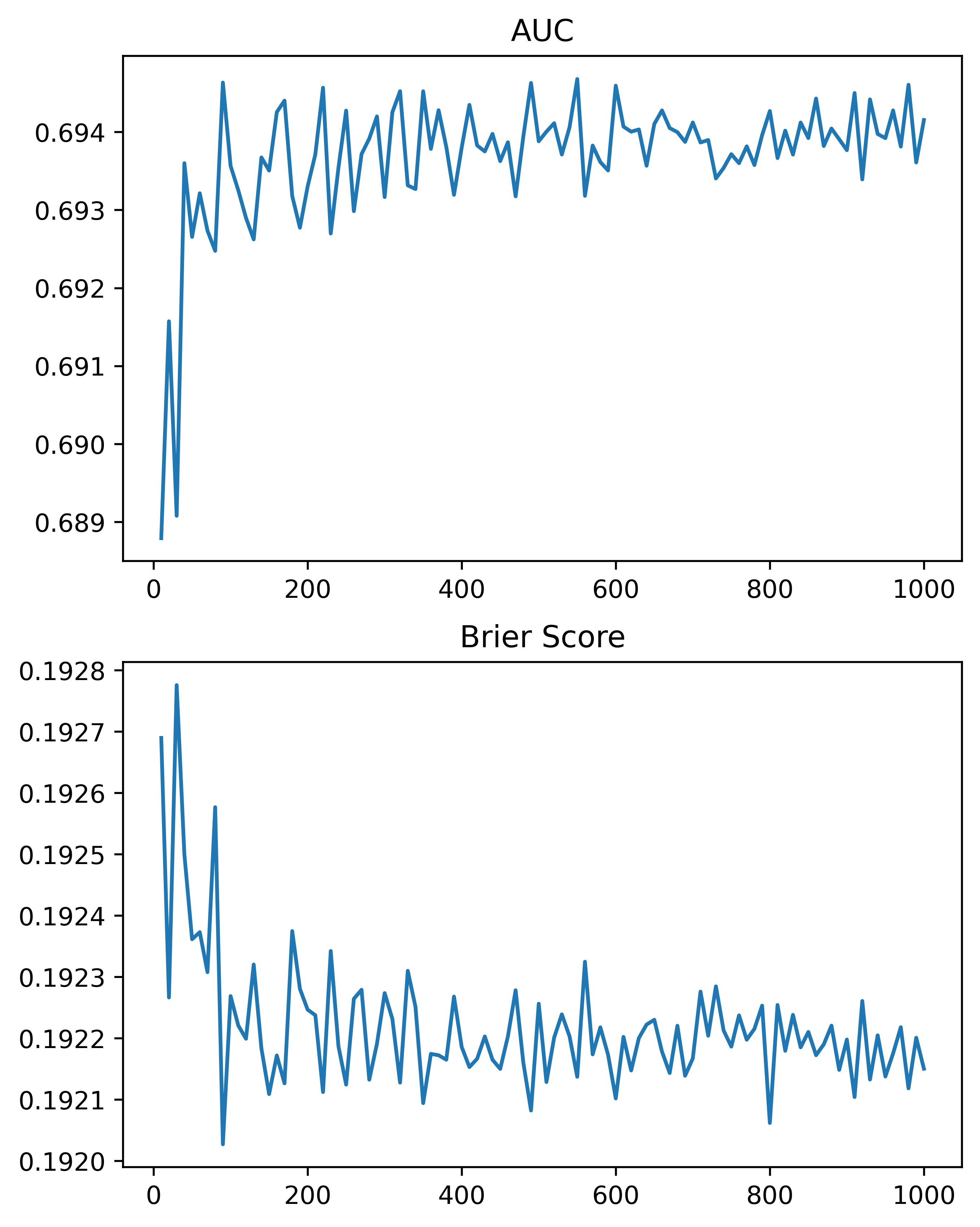
We can see that the relationship is noisy, but the trend clearly decreases with tree size, and perhaps asymptotes post 200 some trees for both metrics in this particular set of data.

So of course it depends on the dataset, but when I see automl libraries choosing trees in the range of 10, 50, 100 for random forests I roll my eyes a bit. You always get more accurate (in a statistical sense), with more trees. You would only choose that few for convenience in fitting and time savings. The R library ranger has a better default of 500 trees IMO (sklearns 100 is often too small in doing tests). But there isn’t much point in trying to hyperparameter tune this – your hyperparameter library may choose a smaller number of trees in a particular run, but this is due to noise in the tuning process itself.

So what metrics do matter for random forests? All machine learning models you need to worry about over-fitting/under-fitting. This depends on the nature of the data (number of rows, can fit more parameters, fewer columns less of opportunity to overfit). Random forests this is dependent on the complexity of the trees – more complex trees can overfit the data. If you have more rows of data, you can fit more complex trees. So typically I am doing searches over (in sklearn parlance) max-depth (how deep a tree can grow), min-samples-split (can grow no more trees is samples are too tiny in a leaf node). Another parameter to search for is how many columns to subsample as well (more columns can find more complex trees).

It can potentially be a balancing act – if you have more samples per leaf, it by default will create less complex trees. Many of the other hyperparameters limiting the complexity of the trees are redundant with these as well (so you could really swap out with max-depth). Here is an example of using the Optuna library a friend recommended to figure out the best parameters for this particular data set, using a train/eval approach (so this splits up the training set even further):

# Consistent train/test split for all evaluations
tr1, tr2 = train_test_split(train, test_size=2000)

def objective(trial):
    param = {
        "n_estimators": 500,
        "max_depth": trial.suggest_int("max_depth", 2, 10),
        "min_samples_split": trial.suggest_int("min_samples_split", 10, 200, step=10),
        "max_features": trial.suggest_int("max_features", 3, 15),
    }
    mod = RandomForestClassifier(**param)
    mod.fit(tr1[recid.xvars], tr1[recid.y1])
    pred_out = mod.predict_proba(tr2[recid.xvars])[:,1]
    auc = roc_auc_score(tr2[recid.y1], pred_out)
    return auc

study = optuna.create_study(direction="maximize")
study.optimize(objective, n_trials=100)
trial = study.best_trial

print(f"Best AUC {trial.value}")
print("Best Params")
print(trial.params)

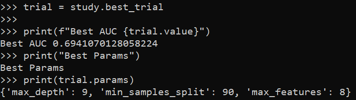
So here it chooses fairly deep trees, 9, but limited complexity via the sample size in a leaf (90). The number of features per tree is alsio slightly larger than default (here 25 features, so default is sqrt(25)). So it appears my personal defaults were slightly under-fitting the data.

My experience regression prefers smaller depth of trees but lower sample sizes (splitting to 1 is OK), but for binary classification limiting sample sizes in trees is preferable.

One thing to pay attention to in these automl libraries, a few do not retrain on the full dataset with the selected hyperparameters. For certain scenarios you don’t want to do this (e.g. if using the eval set to do calibrations/prediction intervals), but if you don’t care about those then you typically want to retrain on the full set. Another random personal observation, random forests really only start to outperform simpler regression strategies at 20k cases, with smaller sample sizes and further splitting train/eval/test, the hyperparameter search is very noisy and mostly a waste of time. If you only have a few hundred cases just fit a reasonable regression model and call it a day.

So here I retrain on the full test set, and then look at the AUC/Brier Score compared to my default model.

# Lets refit according to these params for the full
# training set
mod2 = RandomForestClassifier(n_estimators=500,**trial.params)
mod2.fit(train[recid.xvars], train[recid.y1])
pred_out = mod2.predict_proba(test[recid.xvars])[:,1]
auc_tuned = roc_auc_score(test[recid.y1], pred_out)
bs_tuned = brier_score_loss(test[recid.y1], pred_out)
print(f"AUC tuned {auc_tuned:.4f} vs AUC default {auc[-1]:.4f}")
print(f"Brier Score tuned {bs_tuned:.4f} vs default {bs[-1]:.4f}")

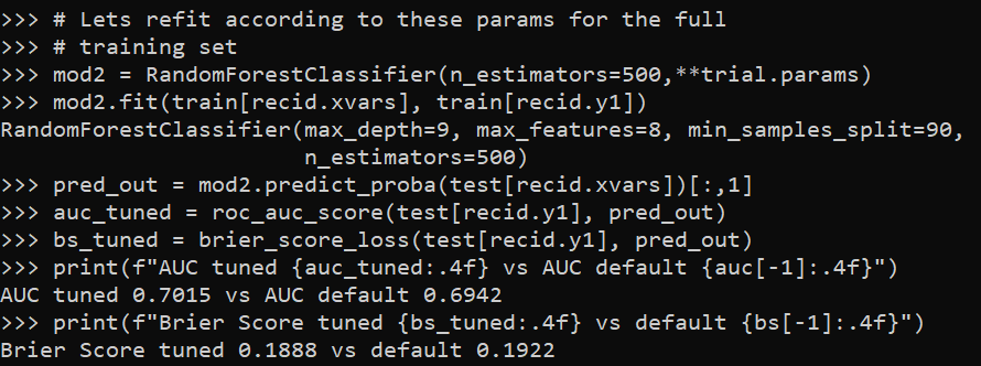
It is definately worth hyperparameter tuning once you have your feature set down, but lift of ~0.01 AUC (which is typical for hypertuned tabular models in my experience) is not a big deal with initial model building. Figuring out a smart way to encode some relevant feature (based on domain knowledge of the problem you are dealing with) typically has more lift than this in my experience.

Prediction Intervals for Random Forests

I previously knew about generating prediction intervals via random forests by calculating the quantiles over the forest. (See this prior python post of mine for getting the individual trees). A recent set of answers on StackExchange show a different approach – apparently the individual tree approach tends to be too conservative (coverage rates higher than you would expect). Those Cross Validated posts have R code, figured it would be good to illustrate in python code how to generate these prediction intervals using random forests.

So first what is a prediction interval? I imagine folks are more familiar with confidence intervals, say we have a regression equation y = B1*x + e, you often generate a confidence interval around B1. Imagine we use that equation to make a prediction though, y_hat = B1*(x=10), here prediction intervals are errors around y_hat, the predicted value. They are actually easier to interpret than confidence intervals, you expect the prediction interval to cover the observations a set percentage of the time (whereas for confidence intervals you have to define some hypothetical population of multiple measures).

Prediction intervals are often of more interest for predictive modeling, say I am predicting future home sale value for flipping houses. I may want to generate prediction intervals that cover the value 90% of the time, and only base my decisions to buy based on the much lower value (if you are more risk averse). Imagine I give you the choice of buy a home valuated at 150k - 300k after flipped vs a home valuated at 230k-250k, the upside for the first is higher, but it is more risky.

In short, this approach to generate prediction intervals from random forests relies on out of bag error metrics (it is sort of like a for free hold out sample based on the bootstrapping approach random forest uses). And based on the residual distribution, one can generate forecast intervals (very similar to Duan’s smearing).

To illustrate, I will use a dataset of emergency room visits and time it took to see a MD/RN/PA, the NHAMCS data. I have code to follow along here, but I will walk through it in this post (that code has some nice functions for data definitions for the NHAMCS data).

At work I am working on a project related to unnecessary emergency room visits, and I actually went to the emergency room in December (for a Kidney stone). So I am interested here in generating prediction intervals for the typical time it takes to be served in an ER to see if my visit was normal or outlying.

Example Python Code

First for some set up, I import the libraries I am using, and read in the emergency room use data:

import numpy as np
import pandas as pd
from nhanes_vardef import * #variable definitions
from sklearn.ensemble import RandomForestRegressor
from sklearn.model_selection import train_test_split

# Reading in fixed width data
# Can download this data from 
# https://ftp.cdc.gov/pub/Health_Statistics/NCHS/Datasets/NHAMCS/
nh2019 = pd.read_fwf('ED2019',colspecs=csp,header=None)
nh2019.columns = list(fw.keys())

Here I am only going to work with a small set of the potential variables. Much of the information wouldn’t make sense to use as predictors of time to first being seen (such as subsequent tests run). One thing I was curious about though was if I changed my pain scale estimate would I have been seen sooner!

# WAITTIME
# PAINSCALE [- missing]
# VDAYR [Day of Week]
# VMONTH [Month of Visit]
# ARRTIME [Arrival time of day]
# AGE [top coded at 95]
# SEX [1 female, 2 male]
# IMMEDR [triage]
#  9 = Blank
#  -8 = Unknown
#  0 = ‘No triage’ reported for this visit but ESA does conduct nursing triage
#  1 = Immediate
#  2 = Emergent
#  3 = Urgent
#  4 = Semi-urgent
#  5 = Nonurgent
#  7 = Visit occurred in ESA that does not conduct nursing triage 

keep_vars = ['WAITTIME','PAINSCALE','VDAYR','VMONTH','ARRTIME',
             'AGE','SEX','IMMEDR']
nh2019 = nh2019[keep_vars].copy()

Many of the variables encode negative values as missing data, so here I throw out visits with a missing waittime. I am lazy though and the rest I keep as is, with enough data random forests should sort out all the non-linear effects no matter how you encode the data. I then create a test split to evaluate the coverage of my prediction intervals out of sample for 2k test samples (over 13k training samples).

# Only keep wait times that are positive
mw = nh2019['WAITTIME'] >= 0
print(nh2019.shape[0] - mw.sum()) #total number missing
nh2019 = nh2019[mw].copy()

# Test hold out sample to show
# If coverage is correct
train, test = train_test_split(nh2019, test_size=2000, random_state=10)
x = keep_vars[1:]
y = keep_vars[0]

Now we can fit our random forest model, telling python to keep the out of bag estimates.

# Fitting the model on training data
regr = RandomForestRegressor(n_estimators=1000,max_depth=7,
  random_state=10,oob_score=True,min_samples_leaf=50)
regr.fit(train[x], train[y])

Now we can use these out of bag estimates to generate error intervals around our predictions based on the test oob error distribution. Here I generate 50% prediction intervals.

# Generating the error distribution
resid = train[y] - regr.oob_prediction_
# 50% interval
lowq = resid.quantile(0.25)
higq = resid.quantile(0.75)
print((lowq,higq)) 
# negative much larger
# so tends to overpredict time

Even 50% here are quite wide (which could be a function of both the data has a wide variance as well as the model is not very good). But we can test whether our prediction intervals are working correctly by seeing the coverage on the out of sample test data:

# Generating predictions on out of sample data
test_y = regr.predict(test[x])
lowt = (test_y + lowq).clip(0) #cant have negative numbers
higt = (test_y + higq)

cover = (test[y] >= lowt) & (test[y] <= higt)
print(cover.mean())

Pretty much spot on. So lets see what the model predicts my referent 50% prediction interval would be (I code myself a 2 on the IMMEDR scale, as I was billed a CPT code 99284, which those should line up pretty well I would think):

# Seeing what my referent time would be
myt = np.array([[6,4,12,930,36,2,6]])
mp = regr.predict(myt)
print(mp)
print( (mp+lowq).clip(0), (mp+higq) )

So a predicted mean of 35 minutes, and a prediction interval of 4 to 38 minutes. (These intervals based on the residual quantiles are basically non-parametric, and don’t have any strong assumptions about the distribution of the underlying data.)

To first see the triage nurse it probably took me around 30 minutes, but to actually be treated it was several hours long. (I don’t think you can do that breakdown in this dataset though.)

We can do wider intervals, here is a screenshot for 80% intervals:

You can see that they are quite wide, so probably not very effective in identifying outlying cases. It is possible to make them thinner with a better model, but it may just be the variance is quite wide. For folks monitoring time it takes for things (whether time to respond to calls for service for police, or here be served in the ER), it probably makes sense to build models focusing on quantiles, e.g. look at median time served instead of mean.

Using Random Forests in ArcPro to forecast hot spots

So awhile back had a request about how to use the random forest tool in ArcPro for crime prediction. So here I will show how to set up the data in a way to basically replicate how I used random forests in this paper, Mapping the Risk Terrain for Crime using Machine Learning. ArcPro is actually pretty nice to replicate how I set it up in that paper to do the models, but I will discuss some limitations at the end.

I am not sharing the whole project, but the data I use you can download from a prior post of mine, RTM Deep Learning style. So here is my initial data set up based on the spreadsheets in that post. So for original data I have crimes aggregated to street units in DC Prepped_Crime.csv (street units are midpoints in street blocks and intersections), and then point dataset tables of alcohol outlet locations AlcLocs.csv, Metro entrances MetroLocs.csv, and 311 calls for service Calls311.csv.

I then turn those original csv files into several spatial layers, via the display XY coordinates tool (these are all projected data FYI). On top of that you can see I have two different kernel density estimates – one for 311 calls for service, and another for the alcohol outlets. So the map is a bit busy, but above is the basic set of information I am working with.

For the crimes, these are the units of analysis I want to predict. Note that this vector layer includes spatial units of analysis even with 0 crimes – this is important for the final model to make sense. So here is a snapshot of the attribute table for my street units file.

Here we are going to predict the Viol_2011 field based on other information, both other fields included in this street units table, as well as the other point/kernel density layers. So while I imagine that ArcPro can predict for raster layers as well, I believe it will be easier for most crime analysts to work with vector data (even if it is a regular grid).

Next, in the Analysis tab at the top click the Tools toolbox icon, and you get a bar on the right to search for different tools. Type in random forest – several different tools come up (they just have slightly different GUI’s) – the one I showcase here is the Spatial Stats tools one.

So this next screenshot shows filling in the data to build a random forest model to predict crimes.

  1. in the input training features, put your vector layer for the spatial units you want to predict. Here mine is named Prepped_Crime_XYTableToPoint.
  2. Select the variable to predict, Viol_2011. The options are columns in the input training features layer.
  3. Explanatory Training Variables are additional columns in your vector layer. Here I include the XY locations, whether a street unit is an intersection, and then several different area variables. These variables are all calculated outside of this procedure.

Note for the predictions, if you just have 0/1 data, you can change the variable to predict as categorical. But later on in determining hotspots you will want to use the predicted probability from that output, not the binary final threshold.

For explanatory variables, here it is ok to use the XY coordinates, since I am predicting for the same XY locations in the future. If I fit a model for Dallas, and then wanted to make predictions for Austin, the XY inputs would not make sense. Finally it is OK to also include other crime variables in the predictions, but they should be lagged in time. E.g. I could use crimes in 2010 (either violent/property) to predict violent crimes in 2011. This dataset has crimes in 2012, and we will use that to validate our predictions in the end.

Then we can also include traditional RTM style distance and kernel density inputs as well into the predictions. So we then include in the training distance features section our point datasets (MetroLocs and AlcLocs), and in our training rasters section we include our two kernel density estimates (KDE_311 calls and KernelD_AlcL1 is the kernel density for alcohol outlets).

Going onto the next section of filling out the random forest tool, I set the output for a layer named PredCrime_Test2, and also save a table for the variable importance scores, called VarImport2. The only other default I change is upping the total number of trees, and click on Calculate Uncertainty at the bottom.

My experience with Random Forests, for binary classification problems, it is a good idea to set the minimum leaf size to say 50~100, and the depth of the trees to 5~10. But for regression problems, regulating the trees is not necessarily as big of a deal.

Click run, and then even with 1000 trees this takes less than a minute. I do get some errors about missing data (should not have done the kernel density masked to the DC boundary, but buffered the boundary slightly I think). But in the end you get a new layer, here it is named PredCrime_Test2. The default symbology for the residuals is not helpful, so here I changed it to proportional circles to the predicted new value.

So you would prioritize your hotspots based on these predicted high crime areas, which you can see in the screenshot are close to the historical ranks but not a 100% overlap. Also this provides a potentially bumpy (but mostly smoothed) set of predicted values.

Next what I did was a table join, so I could see the predicted values against the future 2012 violent crime data. This is just a snap shot, but see this blog post about different metrics you can use to evaluate how well the predictions do.

Finally, we saved the variable importance table. I am not a big fan of these, these metrics are quite volatile in my experience. So this shows the sidewalk area and kernel density for 311 calls are the top two, and the metro locations distance and intersection are at the bottom of variable importance.

But these I don’t think are very helpful in the end (even if they were not volatile). For example even if 311 calls for service are a good predictor, you can have a hot spot without a large number of 311 calls nearby (so other factors can combine to make hotspots have different factors that contribute to them being high risk). So I show in my paper linked at the beginning how to make reduced form summaries for hot spots using shapely values. It is not possible using the ArcPro toolbox (but I imagine if you bugged ESRI enough they would add this feature!).

This example is for long term crime forecasting, not for short term. You could do random forests for short term, such as predicting next week based on several of the prior weeks data. This would be more challenging to automate though in ArcPro environment I believe than just scripting it in R or python IMO. I prefer the long term forecasts though anyway for problem oriented strategies.