The other day on LinkedIn I made a point about how I think scikits TransformedTargetRegressor is very likely to mislead folks. In fact, the example use case in the docs for this function is a common mistake, fitting a model for log(y), then getting predictions phat, and then simply exponentiating those predictions exp(phat).

On LinkedIn I gave an example of how this is problematic for random forests, but here is a similar example for linear regression. For simplicity pretend we only have 3 potential residuals (all equally likely), either a residual of -1, 0, or 1.

Now pretend our logged prediction is 5, so if we simply do exp(5) we get about 148. Now what are our predictions is we consider those 3 potential residuals?

Resid  Pred-Resid Modified_Pred LinPred
  -1     5 - -1        exp(6)     403
   0     5 -  0        exp(5)     148
   1     5 -  1        exp(4)      55

So if we take the mean of our LinPred column, we then get a prediction of about 202. The prediction using this approach is much higher than the naive approach of simply exponentiating 5. The difference is that the exp(5) estimate is the median, and the above estimate taking into account residuals is the mean estimate.

While there are some cases you may want the median estimate, in that case it probably makes more sense to use a quantile estimator of the median from the get go, as opposed to doing the linear regression on log(y). I think for many (probably most) use cases in which you are predicting dollar values, this underestimate can be very problematic. If you are using these estimates for revenue, you will be way under for example. If you are using these estimates for expenses, holy moly you will probably get fired.

This problem will happen for any non-linear transformation. So while some transformations are ok, in scikit for example minmax or standardnormal scalars are ok, things like logs, square roots, or box-cox transformations are not. (To know if it is a linear transformation, if you do a scatterplot of original vs transformed, if it is a straight line it is ok, if it is a curved line it is not!)

I had a friend go back and forth with me for a bit after I posted this. I want to be clear this is not me saying the model of log(y) is the wrong model, it is just to get the estimates for the mean predictions, you need to take a few steps. In particular, one approach to get the mean estimates is to use Duan’s Smearing estimator. I will show how to do that in python below using simulated data.

Example Duan’s Smearing in python

So first, we import the libraries we will be using. And since this is simulated data, will be setting the seed as well.

######################################################
import pandas as pd
import numpy as np
np.random.seed(10)

from sklearn.linear_model import LinearRegression
from sklearn.compose import TransformedTargetRegressor
######################################################

Next I will create a simple linear model on the log scale. So the regression of the logged values is the correct one.

######################################################
# Make a fake dataset, say these are housing prices
n = (10000,1)
error = np.random.normal(0,1,n)
x1 = np.random.normal(10,3,n)
x2 = np.random.normal(5,1,n)
log_y = 10 + 0.2*x1 + 0.6*x2 + error
y = np.exp(log_y)

dat = pd.DataFrame(np.concatenate([y,x1,x2,log_y,error], axis=1),
                   columns=['y','x1','x2','log_y','error'])
x_vars = ['x1','x2']

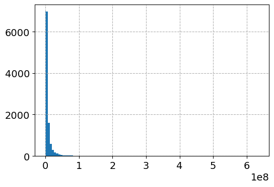
# Lets look at a histogram of y vs log y
dat['y'].hist(bins=100)
dat['log_y'].hist(bins=100)
######################################################

Here is the histogram of the original values:

And here is the histogram of the logged values:

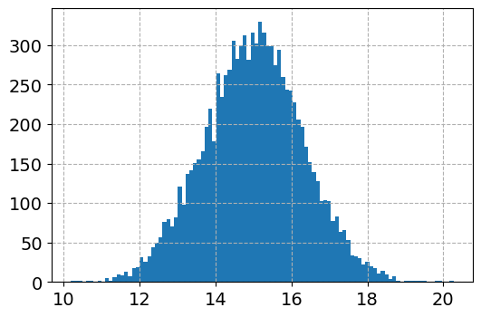
So although the regression is the conditional relationship, if you see histograms like this I would also by default use a regression to predict log(y).

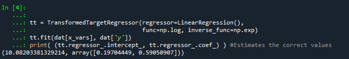
Now here I do the same thing as in the original function docs, I fit a linear regression using the log as the function and exponential as the inverse function.

######################################################
# Now lets see what happens with the usual approach
tt = TransformedTargetRegressor(regressor=LinearRegression(),
                                func=np.log, inverse_func=np.exp)
tt.fit(dat[x_vars], dat['y'])
print( (tt.regressor_.intercept_, tt.regressor_.coef_) ) #Estimates the correct values

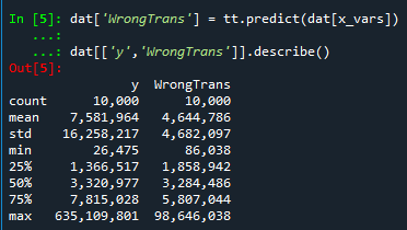
dat['WrongTrans'] = tt.predict(dat[x_vars])

dat[['y','WrongTrans']].describe()
######################################################

So here we estimate the correct simulated values for the regression equation:

But as we will see in a second, the exponentiated predictions are not so well behaved. To illustrate how the WrongTrans variable behaves, I show its distribution compared to the original y value. You can see that on average it is a much smaller estimate. Our sample values have a mean of 7.5 million, and the naive estimate here only has a mean of 4.6 million.

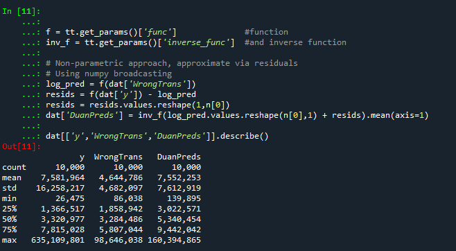
Now here is a way to get an estimate of the mean value. In a nutshell, what you do is take the observed residuals, pretty much like that little table I did in the intro of this blog post, generate predictions given those residuals, and then back transform them and take the mean.

Although this example is using logged regression, I’ve made it pretty general. So if you used any box cox transformation instead of the logged (e.g. sklearns power_transform, it will work.

######################################################
# Duan's smearing, non-parametric approach via residuals

# Can make this general for any function inside of 
# TransformedTargetRegressor
f = tt.get_params()['func']              #function
inv_f = tt.get_params()['inverse_func']  #and inverse function

# Non-parametric approach, approximate via residuals
# Using numpy broadcasting
log_pred = f(dat['WrongTrans'])
resids = f(dat['y']) - log_pred
resids = resids.values.reshape(1,n[0])
dp = inv_f(log_pred.values.reshape(n[0],1) + resids)
dat['DuanPreds'] = dp.mean(axis=1)

dat[['y','WrongTrans','DuanPreds']].describe()
######################################################

So you can see that the Duan Smeared predictions are looking better, at least the mean of the predictions is much closer to the original.

I’ve intentionally done this example without using train/test, as we know the true answers. But in that case, you will want to use the residuals from the training dataset to apply this transformation to the test dataset.

So the residuals and the Duan smearing estimator do not need to be the same dimension. So for example if you have a big data application, you may want to do something like resids = resids.sample(1000) above.

Also another nice perk of this is you can use dp above to give you prediction intervals, so np.quantile(dp,[0.025,0.975], axis=1).T would give you a 95% prediction interval of the mean on the linear scale as well.

Extra, Parametric Estimation

Another approach, which may make sense given the application, is instead of using the observed residuals to give a non-parametric estimate, you can estimate the distribution of the residuals, and then use that to make either an integral estimate of the Smeared estimate back on the original scale. Or in the case of the logged regression there is a closed form solution.

I show how to construct the integral estimator below, again trying to be more general. The integral approach will work for say any box-cox transformation.

######################################################
# Parametric approach, approximating residuals via normal

from scipy.stats import norm
from scipy.integrate import quad

# Look at the residuals again
resids = f(dat['y']) - f(tt.predict(dat[x_vars]))

# Check to make sure that the residuals are really close to normal
# Before doing this
resids.hist(bins=100)

# Fit to a normal distribution 
loc, scale = norm.fit(resids)

# Define integral
def integrand(x,pred):
    return norm.pdf(x, loc, scale)*inv_f(pred - x)

# Pred should be the logged prediction
# -50,50 should be changed if the residuals are scaled differently
def duan_param(pred):
    return quad(integrand, -50, 50, args=(pred))[0]

# This takes awhile to apply to the whole data frame!
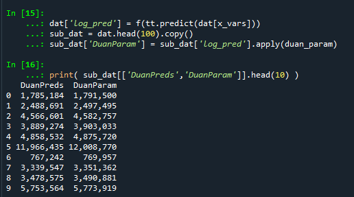
dat['log_pred'] = f(tt.predict(dat[x_vars]))
sub_dat = dat.head(100).copy()
sub_dat['DuanParam'] = sub_dat['log_pred'].apply(duan_param)

# Can see that these are very similar to the non-parametric
print( sub_dat[['DuanPreds','DuanParam']].head(10) )

And you can see that this normal based approximation works just fine here, since by construction the model residuals are pretty well behaved in my simulation.

It happens to be the case that there is a simpler estimate than the integral approach (which you can see in my notes takes awhile to estimate).

###########
# Easier way, but only applicable to log transform
# https://en.wikipedia.org/wiki/Smearing_retransformation
test_val = np.log(5000000)

# Integral approach
print( duan_param(test_val) ) 

# Approach for just log transformed
mult = np.exp(0.5*resids.var())
print( np.exp(test_val)*mult )
##########

So you can see the integral vs the closed form function are very close:

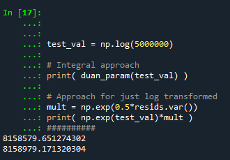
The differences could be due to the the integral is simply an estimate (and you can see I did not do negative to positive infinity, but chopped it off, I do not know if there is a better function to estimate the integral or general approach here).

It wouldn’t surprise me if there are closed form solutions for box-cox transforms as well, but I am not familiar with them offhand. Again the integral approach (or the non-parametric approach) will work for whatever function you want. The function itself could be whatever crazy/discontinuous function you want. But this parametric Duan’s Smearing approach relies on the residuals being normally distributed. (I suppose you could use some other types of continuous distribution estimate if you have reason to, I have only seen normal distribution estimates though in practice.)

Other Notes

While this focuses on regression, I do not think this will perform all that badly for other types of models (such as random forests or xgboost). But for forests it may make sense to simply pull out the individual tree estimates, back transform them, and get the mean of that backtransformed estimate. I have a different blog post that has a function showing how to scoop up the individual predictions from a random forest model.

It should also apply the same to any regression model with regularization. But if you want to do this, there are of course other alternative models you may consider that may be better suited towards your end goals of predictions on the linear/original scale.

For example, if you really want prediction intervals, it may make sense to not transform the data, and estimate a quantile regression model at the 5% and 95% quantiles. This would give you a 90% prediction interval.

Another approach is that it may make sense to use a different model, such as Poisson regression or negative binomial regression (or another generalized linear model in general). Even if your data are not integer counts, you can still use these models! (They just need to be 0 and above, no negative values.)

That Stata blog suggests to use Poisson and then robust standard errors, but that is a bad idea if you are really interested in predictions as well (see Gary Kings comment and linked paper). But you can just do negative binomial models in most cases then, and that is a better default than Poisson for many real world datasets.