Negative Binomial regression and predicted probabilities in SPSS

For my dissertation I have been estimating negative binomial regression models predicting the counts of crimes at small places (i.e. street segments and intersections). When evaluating the fit of poisson regression models and their variants, you typically make a line plot of the observed percent of integer values versus the predicted percent by the models. This is particularly pertinent for data that have a high proportion of zeros, as the negative binomial may still under-predict the number of zeros.

I mistakenly thought that to make such a plot you could simply estimate the predicted value following the negative binomial regression model and then round the predictions. But I was incorrect, and to make the typical predicted versus observed plot you need to estimate the probability of an observation taking an integer value, and then take the mean of that probability over all the observations. That mean will subsequently be the predicted percent given the model. Fortunately I caught my mistake before I gave some talks on my work recently, and I will show how to make said calculations in SPSS. I have posted the data to replicate this work at this dropbox link, and so you can download the data and follow along.

First, I got some help on how to estimate the predicted probabilities via an answer to my question at CrossValidated. So that question lists the formula one needs to estimate the predicted probability for any integer value N after the negative binomial model. To calculate that value though we need to make some special SPSS functions, the factorial and the complete gamma function. Both have SPSS tech help pages showing how to calculate them.

For the factorial we can use a general relationship with the LNGAMMA function.


DEFINE !FACT (!POSITIONAL = !ENCLOSE("(",")"))
( EXP(LNGAMMA((!1)+1)) )
!ENDDEFINE.

And for the complete gamma function we can use a relationship to the CDF of the gamma function.


DEFINE !GAMMAF (!POSITIONAL = !ENCLOSE("(",")"))
( EXP(-1)/(!1)/(CDF.GAMMA(1,(!1),1) - CDF.GAMMA(1,(!1)+1,1)) )
!ENDDEFINE.

And given these two functions, we can create a macro that takes as parameters and returns the predicted probability we are interested in:

  • out – new variable name for predicted probability of taking on that integer value
  • PredN – the predicted mean of the variable conditional on the covariates
  • Disp – estimate of the dispersion parameter
  • Int – the integer value being predicted

DEFINE !PredNB (Out = !TOKENS(1)
               /PredN = !TOKENS(1)
                        /Disp = !TOKENS(1)
                        /Int = !TOKENS(1) )
COMPUTE #a = (!Disp)**(-1).
COMPUTE #mu = !PredN.
COMPUTE #Y = !Int.
COMPUTE #1 = (!GAMMAF(#Y + #a))/(!FACT(#Y)*!GAMMAF(#a)).
COMPUTE #2 = (#a/(#a+#mu))**#a.
COMPUTE #3 =  (#mu/(#a + #mu))**#Y.
COMPUTE !Out =  #1*#2*#3.
!ENDDEFINE.

But to make our plot we want to estimate this predicted probability over a range of values, so I created a helper macro that instead of taking only one integer value, takes the end integer value and will calculate the predicted probability of zero through N.


DEFINE !PredNBRange (Num = !TOKENS(1)
                    /Mean = !TOKENS(1)
                    /Disp = !TOKENS(1)
                    /Stub = !TOKENS(1) )
!DO !I = 0 !TO !Num
  !LET !Base = !CONCAT(!Stub,!I)
  !PredNB Out = !Base PredN = !Mean Disp = !Disp Int = !I.
!DOEND 
!ENDDEFINE.

The example data and code I have posted compares these values to the ones predicted from Stata, and shows my function agrees with Stata to about 7 decimal points. I won’t go through all of those commands here, but I will show how to make the predicted proportions plot after you have a vector of predicted probabilities (you can download all of the code and data and the link I reference prior in the post).

So lets say that you have a vector NB0 TO NB8, and these are the predicted probabilities of integer values 0 to 8 for the observations in your dataset. To subsequently get the mean of the predictions, you can use the AGGREGATE command. Having no variables specified on the BREAK subcommand tells SPSS to aggregate over all values in the dataset. Here I export the file to a new dataset named PredNBAgg.


DATASET DECLARE PredNBAgg.
AGGREGATE OUTFILE='PredNBAgg'
  /BREAK = 
  /NB0 TO NB8 = MEAN(NB0 TO NB8).

Now to merge later on to the observed proportions, I will reshape the dataset so the mean values are all in the same column using VARSTOCASES. Here I also make a category for the predicted probability of being 9 or higher (which isn’t typical for these types of plots, but something I believe is useful).


DATASET ACTIVATE PredNBAgg.
COMPUTE NB9_Plus = 1 - SUM(NB0 TO NB8).
VARSTOCASES /MAKE NBPred FROM NB0 TO NB9_Plus /INDEX Int.
COMPUTE Int = Int - 1. /*Index starts at 1 instead of 0 */.

Now I reactivate my original dataset, here named PredNegBin, calculate the binned observed values (with observations 9 and larger recoded to just 9) and then aggregate those values.


DATASET ACTIVATE PredNegBin.
RECODE TotalCrime (9 THRU HIGHEST = 9)(ELSE = COPY) INTO Int.
DATASET DECLARE PredObsAgg.
AGGREGATE OUTFILE='PredObsAgg'
  /BREAK = Int
  /TotalObs = N.

To get the predicted proportions within each category, I need to do another aggregation to get the total number of observations, and then divide the totals of each integer value with the total number of observations.


DATASET ACTIVATE PredObsAgg.
AGGREGATE OUTFILE = * MODE=ADDVARIABLES OVERWRITE=YES
  /BREAK = 
  /TotalN=SUM(TotalObs).
COMPUTE PercObs = TotalObs / TotalN.

Now we can go ahead and merge the two aggregated datasets together. I also go ahead and close the old PredNBAgg dataset and define a value label so I know that the 9 integer category is really 9 and larger.


MATCH FILES FILE = *
  /FILE = 'PredNBAgg'
  /BY Int.
DATASET CLOSE PredNBAgg.
VALUE LABELS Int 9 '9+'.

Now at this point you could make the plot with the predicted and observed proportions in seperate variables, but this would take two ELEMENT statements within a GGRAPH command (and I like to make line plots with both the lines and points, so it would actually take 4 ELEMENT statements). So what I do here is reshape the data one more time with VARSTOCASES, and make a categorical variable to identify if the proportion is the observed value or the predicted value from the model. Then you can make your chart.


VARSTOCASES /MAKE Dens FROM PercObs NBPred /Index Type /DROP TotalObs TotalN.
VALUE LABELS Type 
 1 'Observed'
 2 'Predicted'.
GGRAPH
  /GRAPHDATASET NAME="graphdataset" VARIABLES=Int Dens Type
  /GRAPHSPEC SOURCE=INLINE.
BEGIN GPL
  SOURCE: s=userSource(id("graphdataset"))
  DATA: Int=col(source(s), name("Int"), unit.category())
  DATA: Type=col(source(s), name("Type"), unit.category())
  DATA: Dens=col(source(s), name("Dens"))
  GUIDE: axis(dim(1), label("Total Crimes on Street Units"))
  GUIDE: axis(dim(2), label("Percent of Streets"))
  GUIDE: legend(aesthetic(aesthetic.color.interior), null())
  SCALE: cat(aesthetic(aesthetic.color.interior), map(("1",color.black),("2",color.red)))
  ELEMENT: line(position(Int*Dens), color.interior(Type))
  ELEMENT: point(position(Int*Dens), color.interior(Type), color.exterior(color.white), size(size."7"))
END GPL.

And voila, here you can see the predicted values are so close to the observed that it is difficult to even see the observed values. Here instead of creating a legend I manually added labels to the chart. A better chart may be to subtract the observed from predicted (especially if you were comparing multiple poisson models), but it should be quite plain to see that the negative binomial fits quite well to the observed data in this instance.

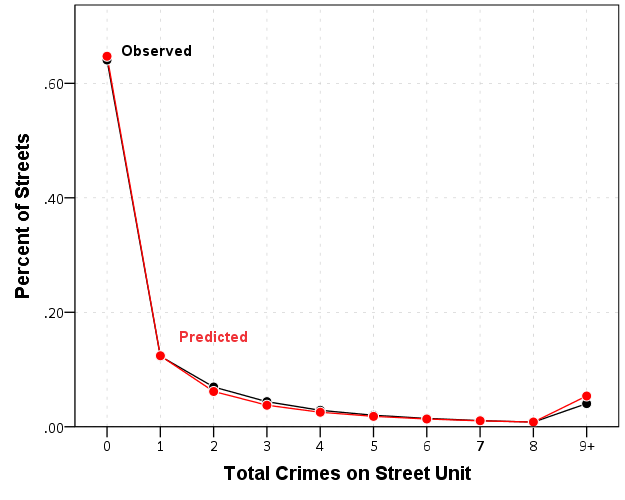
Similar to Paul Allison’s experience, even with nearly 64% of the observations being zero, the negative binomial model fits just fine. I recently fit some other models with the same data (but a different outcome) in which the number of zeros were nearer to 90%. In that instance the negative binomial model would not converge, so estimating a zero inflated model was necessary. Here though it is clearly not necessary, and I would prefer the negative binomial model over a zip (or hurdle) as I see no obvious reason why I would prefer the complications of the different predicted zero equation in addition to the count equation.

Quick SPSS tip: Suppressing output

When running commands in SPSS, it routes summaries and output of particular functions to the active Output document. This is very nice for statistical reporting of various tables, like crosstabs or frequencies or nested regression models. This however is not so nice in some circumstances in which the tables are very big. Rendering the output of these large tables takes a fair bit of memory. Also it is near impossible to navigate the tables when they get very large. (I should note SPSS does have some nice pivot table functionality for nested tables, e.g. in CTABLES, but the examples that follow with don’t apply to that.)

A few examples I come across tables being annoying often are:

  • Large correlation matrices or distance matrices (which I often export directly to an SPSS file – note PROXIMITIES has the option to suppress the table on the command, CORRELATIONS does not).
  • Macro commands that have various data transformations and may produce a series of tables (e.g. VARSTOCASES or CREATE). The regression procedures tend to be the worst offenders, so if you say want the predicted values from a REGRESSION or covariances from FACTOR you get half a dozen other tables along with it.
  • Using SPLIT FILE with many groups.

There are basically two ways I know of to easily suppress the output:

  • Use the Output Management System (OMS)
  • Use SET RESULTS OFF ERRORS OFF. – Via David Marso

It is pretty simple to use either to just suppress the output. For OMS it would be:


OMS /SELECT ALL EXCEPT = [WARNINGS] 
    /DESTINATION VIEWER = NO 
    /TAG = 'NoJunk'.
*Your Commands here.
OMSEND TAG = 'NoJunk'.

The OMS command just grabs all output except for warnings and tells SPSS to not send it to the output viewer. Per some comments I updated the example to take a TAG subcommand on the OMS command, as this allows you to have multiple OMS statements and only turn off specific ones at a time. Here it is hard to see the utility, but it should be more obvious when we place this inside a macro.

To replace the OMS example with the SET RESULTS OFF ERRORS OFF. trick by David Marso, you would basically just replace the original OMS command and then wrap it in PRESERVE and RESTORE statements.


PRESERVE.
SET RESULTS OFF ERRORS OFF.
*Your Commands here.
RESTORE.

Because this changes the system output settings, it is always a good idea to use PRESERVE and then set the user settings back to what they originally were with RESTORE. OMS has the slight advantage here that you can set it to still print warning messages. (I do not know off-hand which version of SPSS the OMS command was introduced.)

I will give a pretty simple example of using OMS with CORRELATIONS to suppress such junk output. A question on SO the other day asked about producing all pair-wise correlations above a threshold, and I gave an answer and an example macro to accomplish this (FYI such things would be useful for producing corrgrams or a network diagram of correlations). The output in that example though still produces the correlation table (which in the original posters situation would produce a 200*200 table in the output) and will produce various junk when running the VARSTOCASES command. Here I wrap the macro in the OMS statement suppressing the tables and you do not get such junk.


DEFINE !CorrPairs (!POSITIONAL !CMDEND)
OMS /SELECT ALL EXCEPT = [WARNINGS] 
    /DESTINATION VIEWER = NO 
    /TAG = "CorrPairs".
DATASET DECLARE Corrs.
CORRELATIONS  /VARIABLES=!1  /MATRIX=OUT('Corrs'). 
DATASET ACTIVATE Corrs.
SELECT IF ROWTYPE_ = "CORR".
COMPUTE #iter = 0.
DO REPEAT X = !1.
  COMPUTE #iter = #iter + 1.
  IF #iter > ($casenum-1) X = $SYSMIS.
END REPEAT.
VARSTOCASES /MAKE Corr FROM !1 /INDEX X2 (Corr) /DROP ROWTYPE_.
RENAME VARIABLES (VARNAME_ = X1).
OMSEND TAG="CorrPairs".
!ENDDEFINE.

And now using the same example data as I used on the question:


***********************************.
*Making fake data.
set seed 5.
input program.
loop i = 1 to 100.
end case.
end loop.
end file.
end input program.
dataset name test.
compute #base = RV.NORMAL(0,1).
vector X(20).
loop #i = 1 to 20.
compute X(#i) = #base*(#i/20)  + RV.NORMAL(0,1).
end loop.
exe.
***********************************.
*Now generate correlation pairs.
!CorrPairs X1 to X20.

If you want to see all the output that was originally generated just comment out the two lines with the OMS and OMSEND statements in the macro. Newer versions of SPSS limit the number of rows displayed in output tables, so your system shouldn’t crash with newer versions of SPSS even when you have enormous tables. But the advice here still applies, as you might as well route the output for those large tables somewhere else so that they are easier to explore (either using OMS to save the tables or helper functions on certain commands to export tables).

Network Xmas Tree in SPSS

Motivated by Rick Wicklin’s raster based Christmas Tree in SAS, here I will show how to lay out a network Xmas tree in SPSS – XKCD network style.

SPSS’s GPL language has the ability to lay out different network diagrams given a list of edges and vertices. One of the layouts is a tree layout, and is intended for hierarchical data. Dendrograms created from hierarchical clustering are some of the most popular uses for this type of layout.

So to create the data for our Xmas tree, what I first did was just drew the XKCD tree on a piece of paper, and then replaced the ornaments with an integer value used to represent a node. Below is my best ASCII art representation of that tree.


              1
          ____|______
         |           |
         2           3
     ____|      _____|_____
    |          |           |
    4          5           6
 ___|____      |       ____|____
|        |     |      |         |
7        8     9     10        11
|_____      ___|___   |         |         
|     |    |       |  |         |
12   13    14      15 16       17

From here we can make an edge dataset that consists of the form of all the directed connections in the above graph. So 1 is connected to 2, 2 is connected to 4 etc. That dataset will look like below.


data list free / XFrom XTo.
begin data
1 2
1 3
2 4
3 5
3 6
4 7
4 8
5 9
6 10
6 11
7 12
7 13
9 14
9 15
10 16
11 17
end data.
dataset name edges.

If all I wanted to do was to draw the edges this would be sufficient for the graph. But I also want to style the nodes, so I create a dataset listing the nodes and a color which I will draw them with.


data list free / Node (F2.0) Type (A15).
begin data
1 Yellow
2 Red
3 Red
4 Green
5 Red
6 Red
7 Red
8 Red
9 Red
10 Green
11 Green
12 Green
13 Red
14 Green
15 Red
16 Green
17 Red
end data.
dataset name nodes.

Now here is the magic of GPL to draw our Xmas tree.


GGRAPH
  /GRAPHDATASET NAME="edges" DATASET = "edges" VARIABLES=XFrom XTo
  /GRAPHDATASET NAME="nodes" DATASET = "nodes" VARIABLES=Node Type
  /GRAPHSPEC SOURCE=INLINE.
BEGIN GPL
 SOURCE: e=userSource(id("edges"))
 DATA: XFrom=col(source(e), name("XFrom"), unit.category())
 DATA: XTo=col(source(e), name("XTo"), unit.category())
 SOURCE: n=userSource(id("nodes"))
 DATA: Node=col(source(n), name("Node"), unit.category())
 DATA: Type=col(source(n), name("Type"), unit.category())
 GUIDE: axis(dim(1), null())
 GUIDE: legend(aesthetic(aesthetic.color.interior), null())
 COORD: rect(dim(1,2), reflect(dim(2)))
 SCALE: cat(aesthetic(aesthetic.color.interior), map(("Yellow", color.yellow), ("Red", color.red), ("Green", color.green)))
 ELEMENT: edge(position(layout.tree(node(Node),from(XFrom), to(XTo), root("1"))))
 ELEMENT: point(position(layout.tree(node(Node),from(XFrom), to(XTo), root("1"))), color.interior(Type), size(size."14"))
END GPL.

I ended up drawing the Y axis (and reflecting it) because my chart template did not have enough padding for the root node and the yellow circle was partially cut off in the plot. I then post-hoc deleted the Y axis, changed the aspect ratio and the background color of the plot. And Voila – Happy Holidays!

Equal Probability Histograms in SPSS

The other day on NABBLE an individual asked for displaying histograms with unequal bar widths. I showed there if you have the fences (and the height of the bar) you can draw the polygons in inline GPL using a polygon element and the link.hull option for edges. I used a similar trick for spineplots.

On researching when someone would use unequal bar widths a common use is to make the fences at specified quantiles and plot the density of the distribution. That is the area of the bars in the plot is equal, but the width varies giving the bars unequal height. Nick Cox has an awesome article about graphing univariate distributions in Stata with equally awesome discussion of said equal probability histograms.

The full code is at the end of the post, but in a nutshell you can call the !EqProbHist MACRO by specifying the Var and how many quantiles to slice it, NTiles. The macro just uses OMS to capture the table of NTiles produced by FREQUENCIES along with the min and max, and returns a dataset named FreqPoly with the lower and upper fences plus the height of the bar. This dataset can then be plotted with a seperate GGRAPH command.

!EqProbHist Var = X NTiles = 25.
GGRAPH
  /GRAPHDATASET DATASET = 'FreqPoly' NAME="graphdataset" VARIABLES=FenceL FenceU Height
  /GRAPHSPEC SOURCE=INLINE.
BEGIN GPL
 SOURCE: s=userSource(id("graphdataset"))
 DATA: FenceL=col(source(s), name("FenceL"))
 DATA: FenceU=col(source(s), name("FenceU"))
 DATA: Height=col(source(s), name("Height"))
 TRANS: base=eval(0)
 TRANS: casenum = index() 
 GUIDE: axis(dim(1), label("X"))
 GUIDE: axis(dim(2), label("Density"))
 SCALE: linear(dim(2), include(0))
 ELEMENT: polygon(position(link.hull((FenceL + FenceU)*(base + Height))), color.interior(color.grey), split(casenum)) 
END GPL.

An example histogram is below.

Note if you have quantiles that are tied (e.g you have categorical or low count data) you will get division by zero errors. So this type of chart is only reasonable with continuous data.

*********************************************************************************************.
*Defining Equal Probability Macro - only takes variable and number of tiles to slice the data.
DEFINE !EqProbHist (Var = !TOKENS(1)
                   /NTiles = !TOKENS(1) )
DATASET DECLARE FreqPoly.
OMS
/SELECT TABLES
/IF SUBTYPES = 'Statistics'
/DESITINATION FORMAT = SAV OUTFILE = 'FreqPoly' VIEWER = NO.
FREQUENCIES VARIABLES=!Var
  /NTILES = !NTiles
  /FORMAT = NOTABLE
  /STATISTICS = MIN MAX.
OMSEND.
DATASET ACTIVATE FreqPoly.
SELECT IF Var1 <> "N".
SORT CASES BY Var4.
COMPUTE FenceL = LAG(Var4).
RENAME VARIABLES (Var4 = FenceU).
COMPUTE Height = (1/!NTiles)/(FenceU - FenceL).
MATCH FILES FILE = *
/KEEP FenceL FenceU Height.
SELECT IF MISSING(FenceL) = 0.
!ENDDEFINE.
*Example Using the MACRO and then making the graph.
dataset close all.
output close all.
set seed 10.
input program.
loop #i = 1 to 10000.
  compute X = RV.LNORMAL(1,0.5).
  compute X2 = RV.POISSON(3).
  end case.
end loop.
end file.
end input program.
dataset name sim.
PRESERVE.
SET MPRINT OFF.
!EqProbHist Var = X NTiles = 25.
GGRAPH
  /GRAPHDATASET DATASET = 'FreqPoly' NAME="graphdataset" VARIABLES=FenceL FenceU Height
  /GRAPHSPEC SOURCE=INLINE.
BEGIN GPL
 SOURCE: s=userSource(id("graphdataset"))
 DATA: FenceL=col(source(s), name("FenceL"))
 DATA: FenceU=col(source(s), name("FenceU"))
 DATA: Height=col(source(s), name("Height"))
 TRANS: base=eval(0)
 TRANS: casenum = index() 
 GUIDE: axis(dim(1), label("X"))
 GUIDE: axis(dim(2), label("Density"))
 SCALE: linear(dim(2), include(0))
 ELEMENT: polygon(position(link.hull((FenceL + FenceU)*(base + Height))), color.interior(color.grey), split(casenum)) 
END GPL.
RESTORE.
*********************************************************************************************.

Stacked (pyramid) bar charts for Likert Data

A while ago this question on Cross Validated showed off some R libraries to plot Likert data. Here is a quick post on replicating the stacked pyramid chart in SPSS.

This is one of the (few) examples where stacked bar charts are defensible. One task that is easier with stacked bars (and Pie charts – which can be interpreted as a stacked bar wrapped in a circle) is to combine the lengths of adjacent categories. Likert items present an opportunity with their ordinal nature to stack the bars in a way that allows one to more easily migrate between evaluating positive vs. negative responses or individually evaluating particular anchors.

First to start out lets make some fake Likert data.

**************************************.
*Making Fake Data.
set seed = 10.
input program.
loop #i = 1 to 500.
compute case = #i.
end case.
end loop.
end file.
end input program.
dataset name sim.
execute.
*making 30 likert scale variables.
vector Likert(30, F1.0).
do repeat Likert = Likert1 to Likert30.
compute Likert = TRUNC(RV.UNIFORM(1,6)).
end repeat.
execute.
value labels Likert1 to Likert30 
1 'SD'
2 'D'
3 'N'
4 'A'
5 'SA'.
**************************************.

To make a similar chart to the one posted earlier, you need to reshape the data so all of the Likert items are in one column.

**************************************.
varstocases
/make Likert From Likert1 to Likert30
/index Question (Likert).
**************************************.

Now to make the population pyramid Likert chart we will use SPSS’s ability to reflect panels, and so we assign an indicator variable to delineate the positive and negative responses.

***************************************
*I need to make a variable to panel by.
compute panel = 0.
if Likert > 3 panel = 1.
***************************************.

From here we can produce the chart without displaying the neutral central category. Here I use a temporary statement to not plot the neutral category, and after the code is the generated chart.

***************************************.
temporary.
select if Likert <> 3.
GGRAPH
  /GRAPHDATASET NAME="graphdataset" VARIABLES=Question COUNT()[name="COUNT"] Likert panel
    MISSING=LISTWISE REPORTMISSING=NO
  /GRAPHSPEC SOURCE=INLINE.
BEGIN GPL
  SOURCE: s=userSource(id("graphdataset"))
  COORD: transpose(mirror(rect(dim(1,2))))
  DATA: Question=col(source(s), name("Question"), unit.category())
  DATA: COUNT=col(source(s), name("COUNT"))
  DATA: Likert=col(source(s), name("Likert"), unit.category())
  DATA: panel=col(source(s), name("panel"), unit.category())
  GUIDE: axis(dim(1), label("Question"))
  GUIDE: axis(dim(2), label("Count"))
  GUIDE: axis(dim(3), null(), gap(0px))
  GUIDE: legend(aesthetic(aesthetic.color.interior), label("Likert"))
  SCALE: linear(dim(2), include(0))
  SCALE: cat(aesthetic(aesthetic.color.interior), sort.values("1","2","5","4"), map(("1", color.blue), ("2", color.lightblue), ("4", color.lightpink), ("5", color.red)))
  ELEMENT: interval.stack(position(Question*COUNT*panel), color.interior(Likert), shape.interior(shape.square))
END GPL.
***************************************.

These charts when displaying the Likert responses typically allocate the neutral category half to one panel and half to the other. To accomplish this task I made a continuous random variable and then use the RANK command to assign half of the cases to the positive panel.

***************************************.
compute rand = RV.NORMAL(0,1).
AUTORECODE  VARIABLES=Question  /INTO QuestionN.
RANK
  VARIABLES=rand  (A) BY QuestionN Likert /NTILES (2)  INTO RankT /PRINT=NO
  /TIES=CONDENSE .
if Likert = 3 and RankT = 2 panel = 1.
***************************************.

From here it is the same chart as before, just with the neutral category mapped to white.

***************************************.
GGRAPH
  /GRAPHDATASET NAME="graphdataset" VARIABLES=Question COUNT()[name="COUNT"] Likert panel
    MISSING=LISTWISE REPORTMISSING=NO
  /GRAPHSPEC SOURCE=INLINE.
BEGIN GPL
  SOURCE: s=userSource(id("graphdataset"))
  COORD: transpose(mirror(rect(dim(1,2))))
  DATA: Question=col(source(s), name("Question"), unit.category())
  DATA: COUNT=col(source(s), name("COUNT"))
  DATA: Likert=col(source(s), name("Likert"), unit.category())
  DATA: panel=col(source(s), name("panel"), unit.category())
  GUIDE: axis(dim(1), label("Question"))
  GUIDE: axis(dim(2), label("Count"))
  GUIDE: axis(dim(3), null(), gap(0px))
  GUIDE: legend(aesthetic(aesthetic.color.interior), label("Likert"))
  SCALE: linear(dim(2), include(0))
  SCALE: cat(aesthetic(aesthetic.color.interior), sort.values("1","2","5","4", "3"), map(("1", color.blue), ("2", color.lightblue), ("3", color.white), ("4", color.lightpink), ("5", color.red)))
  ELEMENT: interval.stack(position(Question*COUNT*panel), color.interior(Likert),shape.interior(shape.square))
END GPL.
***************************************.

The colors are chosen to illustrate the ordinal nature of the data, with the anchors having a more saturated color. To end I map the neutral category to a light grey and then omit the outlines of the bars in the plot. They don’t really add anything (except possible moire patterns), and space is precious with so many items.

***************************************.
GGRAPH
  /GRAPHDATASET NAME="graphdataset" VARIABLES=Question COUNT()[name="COUNT"] Likert panel
    MISSING=LISTWISE REPORTMISSING=NO
  /GRAPHSPEC SOURCE=INLINE.
BEGIN GPL
  SOURCE: s=userSource(id("graphdataset"))
  COORD: transpose(mirror(rect(dim(1,2))))
  DATA: Question=col(source(s), name("Question"), unit.category())
  DATA: COUNT=col(source(s), name("COUNT"))
  DATA: Likert=col(source(s), name("Likert"), unit.category())
  DATA: panel=col(source(s), name("panel"), unit.category())
  GUIDE: axis(dim(1), label("Question"))
  GUIDE: axis(dim(2), label("Count"))
  GUIDE: axis(dim(3), null(), gap(0px))
  GUIDE: legend(aesthetic(aesthetic.color.interior), label("Likert"))
  SCALE: linear(dim(2), include(0))
  SCALE: cat(aesthetic(aesthetic.color.interior), sort.values("1","2","5","4", "3"), map(("1", color.blue), ("2", color.lightblue), ("3", color.lightgrey), ("4", color.lightpink), ("5", color.red)))
  ELEMENT: interval.stack(position(Question*COUNT*panel), color.interior(Likert),shape.interior(shape.square),transparency.exterior(transparency."1"))
END GPL.
***************************************.

Cyclical color ramps for time series line plots

Morphet & Symanzik (2010) propose different novel cyclical color ramps by taking ColorBrewer ramps and wrapping them on the circle. All other previous continuous circle ramps I had seen prior were always rainbow scales, and there is plenty discussion about why rainbow color scales are bad so we needn’t rehash that here (see Kosara, Drew Skau, and my favorite Why Should Engineers and Scientists Be Worried About Color? for a sampling of critiques).

Below is a picture of the wrapped cyclical ramps from Morphet & Symanzik (2010). Although how they "average" the end points is not real clear to me from reading the paper, they basically use a diverging ramp and have one end merge at a fully saturated end of the sprectrum (e.g. nearly black) and the other merge at the fully light end of the spectrum (e.g. nearly white).

The original motivation is for directional data, and here is a figure from my paper Viz. JTC lines comparing the original rainbow color ramp I chose (on the right) and an updated red-grey cyclical scale on the left. The map is still quite complicated, as part of the motivation of that map was to show how plotting the JTC the longer lines dominate the graphic.

But I was interested in applying this logic to showing cyclical line plots, e.g. aoristic crime estimates by hour of day and day of week. Using the same Arlington data I used before, here are the aoristic estimates for hour of day plotted seperately for each day of the week. The colors for the day of the week use SPSS’s default color scheme for nominal categories. SPSS does not have anything as far as color defaults to distinguish between ordinal data, so if you use a categorical coloring scheme this is what you get.

The default is very good to distinguish between nominal categories, but here I want to take advantage of the cyclical nature of the data, so I employ a cyclical color ramp.

From this it is immediately apparent that the percentage of crimes dips down during the daytime for the grey Saturday and Sunday aoristic estimates. Most burglaries happen during the day, and so you can see that when homeowners are more likely to be in the house (as oppossed to at work) burglaries are less likely to occur. Besides this, day of week seems largely irrelevant to the percentage of burglaries that are occurring in Arlington.

I chose to make during the week shades of red, the dark color split between Friday-Saturday, and the light color split between Sunday-Monday. This trades one problem for another, in that the more fully saturated colors draw more attention in the plot, but I believe it is a worthwhile sacrifice in this instance. Below are the Hexidecimal RGB codes I used for each day of the week.

Sun - BABABA
Mon - FDDBC7
Tue - F4A582
Wed - D6604D
Thu - 7F0103
Fri - 3F0001
Sat - 878787

Hanging rootograms and viz. differences in time series

These two quick charting tips are based on the notion that comparing differences from a straight line are easier than comparing deviations from a curved line. The problems with comparing differences between curved lines are similar to the difference between comparings length and distance from a common baseline (so Cleveland’s work is applicable), but the task of comparing two curves comes up enough that it deserves some specific attention.

The first example is comparing differences between a histogram and an estimated distribution. For example, people often like to superimpose a distribution curve on a histogram, and here is an example SPSS chart.

I believe it was Tukey who suggested that instead of plotting the histogram bars at the zero upwards, you hang them from the expected value. What this does is that instead of comparing differences from a curved line, you are comparing differences to the straight reference line at zero.

Although it is usual to plot the bars to cover the entire bin, I sometimes find this distracting. So here is an alternative (in SPSS – with example code linked to at the end of the post) in which I only plot lines and dots and just note in text the bin widths are in-between the hash marks on the X axis.

The second example is taken from William Playfair’s atlas, and Cleveland uses it to show that comparing two curves can be misleading. (It took me forever to find this data already digitized, so thanks for the bissantz blog for posting it.)

Instead of comparing the two curves only in terms of vertical deviations from one another, we tend to compare the curves in terms of the nearest location. Here the visual error in the magnitude of differences is likely to occur in the area between 1760 and 1766, where they look very close to one another because of the upward slope for both time series in that period.

Here I like the default behavior of SPSS when plotting the differences as an interval element and it is easier to see this potential error (just compare the length of the bars). When using a continuous scale, SPSS plots the interval elements with zero area inside and only an exterior outline (which ends up being near equivalent to a edge element).

More frequently though, people suggest just to plot the differences, and here is a chart with all three (Imports, Exports and the difference) plotted on the same graph. Note the differences at 1763 (390) is actually larger than the difference and the start of the series, 280 at 1700.

You can do similar things to scatterplots, which Tukey calls detilting plots. Again, the lesson is it is easier to compare differences from a straight line than it is differences from a curve (or sloped line). Here I have posted the SPSS code to make the graphs (I slightly cheated though and post edited in the guidelines and labels in the graph editor).

Using circular dot plots instead of circular histograms

Although as I mentioned in this post on circular helio bar charts, polar coordinates are unlikely to be as effective as rectilinear coordinates for most types of comparisons, I really wanted to use a circular histogram in a recent paper of mine. The motivation is I have circular data in form of azimuths (Journey to Crime), aggregated to quadrants. So I really wanted to use a small multiple plot of circular histograms with the visual connection to the actual direction the azimuths were distributed within each quadrant.

Part of the problem with circular histograms though is that the area near the center of the plot shrinks to nothing.

So a simple solution is to offset the center of the plot, so the bars don’t start at the origin, but a prespecified distance away from the center of the circle. Below is the same chart previously with a slight offset. (I saw this idea originally in Wilkinson’s Grammar of Graphics.)

And here is that technique extended to an example small multiple histogram from an earlier draft of the paper I previously mentioned.

Even with the offset, the problem of the shrinking area is even worse because of the many plots, and the outlying bars in one plot shrinks the rest of the distribution even more dramatically. So, even with the offsetting it is still quite difficult assess trends. Also note I don’t even bother to draw the radius guide lines. I noticed in some recent papers about analyzing circular data that they don’t draw bars for circular histograms, but use dots (and/or kernel density estimates). See examples in Brunsdon and Corcoran (2006), Ashby and Bowers (2013), and Russell and Levitin (1995). The below image is taken from Ashby and Bowers (2013) to demonstrate this.

The idea behind this is that, in polar coordinates, you need to measure the length of the bar, instead of distance from a common reference line. When you use dots, it is pretty trivial to just count the dots to see how far they stack up (so no axis guide is needed). This just replaces one problem for other ones, especially for larger sample sizes (in which you will need to discretize how many observations a point represents) but I don’t think it is any worse than bars at least in this situation (and can potentially be better for a smaller number of dots). One thing that does happen with points is that large stacks deviate from each other the further they grow towards the circumference of the polar coordinate system (the bars in histograms typically get wider). This just looks aesthetically bad, although the bars growing wider could be considered a disingenuous representation (e.g. Florence Nightingale’s coxcomb chart) (Brasseur, 2005; Friendly, 2008).

Unfortunately, SPSS’s routine to stack the dots in polar coordinates is off just slightly (I have full code linked at the end of the post to recreate some of the graphs in the post and display this behavior).

With alittle data manipulation though you can basically roll your own (although this is fixed bins, unlike irregular ones chosen based on the data like in Wilkinson’s dot plots, e.g. bin.dot in GPL) (Wilkinson, 1999).

And here is the same example small multiple histogram using the dots.

Here I have posted the code to demonstrate some of the graphs here (and I have the full code for the Viz. JTC paper here). To make the circular dot plot I use the sequential case processing trick, and then show how to use TRANS statements in inline GPL to adjust the positioning of the dots and if you want the dots to represent multiple values.


References

Querying Graph Neighbors in SPSS

The other day I showed how one could make an edge list in SPSS, which is needed to generate network graphs. Today, I will show how one can use an edge list in long format to identify neighbors for higher degree relationships.

So to start, what do I mean by a neighbor of higher degree relationship? Lets say I have a relationship between two nodes A B. Now lets also say I have another relationship between nodes B C. I might say that A and C don’t have a direct relationship, but they are related in that they both have a relationship to B. So A is a first degree neighbor of B, and A is a second degree neighbor of C. If I drew a graph of the listed network, the degree relationship between A and C would be the minimum number of edges one would have to traverse to get from the A node to the C node.

A  B  C

Why would a criminologist or crime analyst care about relationships of higher degrees? Well, here are two examples I am familiar with in criminology;

For more simple and practical motivation for crime analysts, you may just have some particular individuals who you want to have targeted enforcement towards (known chronic offenders, violent gang members) and you would like to compile a more extended network of individuals related to those particular offenders to keep an eye on, or further investigate for possible ties to co-offending or gang activity.

So to start in SPSS, lets say that we have a edge list in long format, where there is a column that ID’s each person, and another column that shows if those two people are related at the same event. Exampe ties for a crime analyst may be victimizations, or co-offending, or being stopped for field interviews at the same time.

*Long dataset marking people sharing same incident (ID).
data list free / IncID (F2.0) Person (A15).
begin data
1 John 
1 Mary
2 John 
2 Frank
3 John 
3 William
4 John 
4 Andrew
5 Mary 
5 Frank
6 Mary 
6 William
7 Frank 
7 Kelly
8 Andrew 
8 Penny
9 Matt 
9 Andrew
10 Kelly 
10 Andrew
end data.
dataset name long.
dataset activate long.

Now, lets say we want to grab higher degree neighbors for Mary, first I will ID the first degree neighbors by creating a flag, and then aggregating within the incident ID. That is, cases that share an incident with Mary.


*ID Mary and then aggregate to get first degree.
compute degree1 = (Person = "Mary").
*Now aggregate to get all degree1s.
AGGREGATE
  /OUTFILE=* MODE=ADDVARIABLES OVERWRITE = YES
  /BREAK=IncID
  /degree1 = MAX(degree1).

To identify if a person is a second degree neighbor of Mary, I can first aggregate within person, to ID that both John and Frank are first degree neighbors, and then pick their first degree neighbors, who I will then be able to tell are second degree neighbors of Mary.


*Aggregate within edge ID to get second degrees.
AGGREGATE
  /OUTFILE=* MODE=ADDVARIABLES OVERWRITE = YES
  /BREAK=Person
  /degree2 = MAX(degree1).
AGGREGATE
  /OUTFILE=* MODE=ADDVARIABLES OVERWRITE = YES
  /BREAK=IncID
  /degree2 = MAX(degree2).

I can continue to do the same procedure for third degree neighbors.


*Aggregate within edge ID to get third degrees.
AGGREGATE
  /OUTFILE=* MODE=ADDVARIABLES OVERWRITE = YES
  /BREAK=Person
  /degree3 = MAX(degree2).
AGGREGATE
  /OUTFILE=* MODE=ADDVARIABLES OVERWRITE = YES
  /BREAK=IncID
  /degree3 = MAX(degree3).

So now this should be clear how I can make a recursive structure to identify neighbors of however many degrees I want. I end the post with a general MACRO to estimate all neighbors of a certain degree given an edge list in long format. Since this will expand to very many cases, you will likely only want to use a smaller list, or I provided an option in the macro to only check certain flagged individuals for neighbors.

I’d love to see or hear about other applications crime analysts are using such social networks for. On the academic bucket list to learn more about graph layout algorithms, so hopefully you see more posts about that from me in the future.


*Current requirement - personid needs to be a string variable.
*Flag argument will return people who have a value of one for that variable and all of there
neighbors in the long list.
DEFINE !neighbor (incid = !TOKENS(1)
                           /personid = !TOKENS(1)
                           /number = !TOKENS(1) 
                           /flag = !DEFAULT ("") !TOKENS(1)   )

dataset copy neighbor.
dataset activate neighbor.
match files file = *
/keep = !incid !personid !flag.

rename variables (!incid = IncID)
(!personid = Person).

*I need to make a stacked dataset for all cases.
compute XXconstXX = 1.

*Making wide dataset of Persons in the long list.
dataset copy XXwideXX.
dataset activate XXwideXX.

*eliminating duplicate people.
sort cases by Person.
match files file = *
/first = XXkeepXX
/by Person
/drop IncID.
select if XXkeepXX = 1.

*reshaping long to wide - could use flip here but that requires numeric PersonIDs.
*flip variables = Person.
!IF (!flag  !NULL) !THEN
select if !flag = 1.
!IFEND
casestovars
/ID = XXconstXX
/seperator = ""
/drop XXkeepXX !flag.
*Similar here you could just replace with a list of all unique offender nodes - just needs to be in wide format.

*Match back to the original long dataset.
dataset activate neighbor.
match files file = *
/table = 'XXwideXX'
/by XXconstXX.
dataset close XXwideXX.

*Reshape wide to long - @ is for filler so I dont need to know how many people - it gets dropped by default in varstocases.
string @ (A1).
varstocases
/make DegreePers from Person1 to @
/drop XXconstXX !flag.

sort cases by DegreePers IncID Person.

*Make first degree.
compute degree1 = (Person = DegreePers).
AGGREGATE
  /OUTFILE=* MODE=ADDVARIABLES OVERWRITE = YES
  /BREAK=IncID DegreePers
  /degree1 = MAX(degree1).
AGGREGATE
  /OUTFILE=* MODE=ADDVARIABLES OVERWRITE = YES
  /BREAK=Person DegreePers
  /degree1 = MAX(degree1).
*dropping self checks.
select if Person  DegreePers.

!LET !past = "degree1"
!DO !i = 2 !TO !number
!LET !current = !CONCAT("degree",!i)
AGGREGATE
  /OUTFILE=* MODE=ADDVARIABLES OVERWRITE = YES
  /BREAK=IncID DegreePers
  /!current = MAX(!past).
AGGREGATE
  /OUTFILE=* MODE=ADDVARIABLES OVERWRITE = YES
  /BREAK=Person DegreePers
  /!current = MAX(!current).
!LET !past = !current
!DOEND
*Clean up and delete duplicates.
compute degree = (!number + 1) - SUM(degree1 to !current).
string P1 P2 (A100).
DO IF Person <= DegreePers.
    compute P1 = Person.
    compute P2 = DegreePers.
ELSE.
    compute P1 = DegreePers.
    compute P2 = Person.
END IF.
sort cases by P1 P2.
match files file = *
/first = XXkeepXX
/by P1 P2
/drop DegreePers Person.
*will be [1 + degrees searched] if not a neighbor.
select if XXkeepXX = 1 and degree <= !number.
match files file = *
/drop degree1 to !current XXkeepXX IncID.
formats degree (!CONCAT("F",!LENGTH(!number),".0")).
!ENDDEFINE.

*Example use case - uncomment to check it out.
*dataset close ALL.
*Long dataset marking people sharing same incident (ID).
*data list free / IncID (F2.0) Person (A15).
*begin data
1 John 
1 Mary
2 John 
2 Frank
3 John 
3 William
4 John 
4 Andrew
5 Mary 
5 Frank
6 Mary 
6 William
7 Frank 
7 Kelly
8 Andrew 
8 Penny
9 Matt 
9 Andrew
10 Kelly 
10 Andrew
*end data.
*dataset name long.
*dataset activate long.
*compute myFlag = 1.
*set mprint on.
*output close ALL.
*neighbor incid = IncID personid = Person number = 3.
*set mprint off.
*dataset activate long.
*dataset close neighbor.
*compute myFlag = (Person = "Mary" or Person = "Andrew").
*set mprint on.
*output close ALL.
*neighbor incid = IncID personid = Person number = 3 flag = myFlag.
*set mprint off.

Quick SPSS Tip: Cleaning up irregular characters in strings

This is just intended to be a quick tip on cleaning up string fields in SPSS. Frequently if I am parsing a field or matching string records (such as names or addresses) I don’t want extra ascii characters besides names and/or numbers in the field. For example, if I have a name I might want to eliminate hyphens or quotes, or if I have a field that is meant to be a house number I typically do not want any alpha character in the end (geocoding databases will rarely be able to tell the difference between Apt’s 1A and 1B).

We can use a simple loop and the PIB variable format in SPSS to clean out unwanted ascii codes in string characters. So for instance if I wanted to replace all the numbers with nothing in a string field I could use this code below (where OrigField is the original field with the numbers contained, and CleanField is the subsequent cleaned variable).

string CleanField (A5).
compute CleanField = OrigField.
loop #i = 48 to 57.
compute CleanField = REPLACE(CleanField,STRING(#i,PIB),"").
end loop.

The DEC column in the linked ascii table corresponds to the ascii character code in SPSS’s PIB format. The numbers 0 through 9 end up being 48 to 57 in decimal values, so I create a string corresponding to those characters via the string(#i,PIB) commmand and replace them with nothing in the REPLACE command. I loop through values of 48 to 57 to get rid of all numeric values.

This extends to potentially all characters, for instance if I want to return only capital alpha characters, I could use a loop with an if statement like below;

string CleanField (A5).
compute CleanField = OrigField.
loop #i = 1 to 255.
if #i < 65 or #i > 90 CleanField = REPLACE(CleanField,STRING(#i,PIB),"").
end loop.

There are (a lot) more than 255 ascii characters, but that should suffice to clean up most string fields in English.