So hacker news the other day had a thread on how do you test your SQL code. This is such a nerd/professional data science type of question I love it (and many of the high upvoted answers are good, but lack code example/nitty gritty details, hence this blog post). I figured I would make my notes on this and illustrate some real code. You get a few things in this post:
- how to set up spark locally on a windows machine
- how to generate SQL tests in python with pytest
- how to set up a github action CICD pipeline to test pyspark/sql
Setting up spark on Windows
First, before we get start, getting spark up and running on a windows machine is non-trivial. Maybe I should use Docker, like I do for postgres, but here are my notes on setting it up to run locally on Windows (much of this is my condensed notes + a few extras based on this DataCamp post).
- Step 1: Install Java. Make sure where you install it has NO SPACES. Then create an environment variable,
JAVA_HOME, and point it to where you installed Java. Mine for example isC:\java_jdk(no spaces). - Step 2: Install spark. Set the environment variable
Spark_hometo wherever you downloaded it, mine is set toC:\spark. Additionally set the environment variablesPYSPARK_HOMEtopython. - Step 3: Set up your python environment, e.g. something like
conda create --name spenv python=3.9 pip pyspark==3.2.1 pyarrow pandas pytestto follow along with this post. (Note to make pyspark and spark downloaded versions line up.) - Step 4: Then you need to download
winutils.exethat matches your version. So I currently have spark=3.2.1, so I just do a google search for “winutils 3.2” and up pops this github repo with the version I need (minor versions probably don’t matter). (You do not need to double click to install, the exe file just needs to be available for other programs to find.) Then set the environment variablehadoop_hometo the folder where you downloadedwinutils.exe. Mine isC:\winutils.
I know that is alot – but it is a one time thing. Now once this is done, from the command line try to run:
pyspark --versionYou should be greeted with something that looks like:
Welcome to
      ____              __
     / __/__  ___ _____/ /__
    _\ \/ _ \/ _ `/ __/  '_/
   /___/ .__/\_,_/_/ /_/\_\   version 3.2.1
      /_/

Using Scala version 2.12.15, Java HotSpot(TM) 64-Bit Server VM, 11.0.15
Plus a bunch of other messages (related to logging errors on windows). (You can set the spark-defaults.conf and log4j.properties file to make these less obnoxious.)
But now you are good to go running spark locally on your windows machine. Note you get none of the reasons you want to use spark, such as distributing computations over multiple machines (this is equivalent to running computations on the hnode). But is convenient to do what I am going to show – testing your SQL code locally.
Testing SQL code in python
Now that we have pyspark set up, we can run a test in python. Instead of type python into the REPL, go ahead and run pyspark, so we are in a pyspark REPL session. You will again see the big Spark ascii art at the beginning. Here is an example of now creating a dummy temp table inside of our spark database (this is just a local temp table).
# Inside of pyspark REPL
# so spark is available
import pandas as pd

x = [1,2,3,4]
y = ['a','b','c','c']
df = pd.DataFrame(zip(x,y),columns=['x','y'])

# Can create a temp spark table based on fake data
sdf = spark.createDataFrame(df)
sdf.createOrReplaceTempView('test_table')
Now we can run our SQL against the spark database.
# sql to test
query = '''
SELECT
  SUM(x) AS cum_x,
  COUNT(y) AS n,
  y
FROM test_table
GROUP BY y'''

spark.sql(query).show()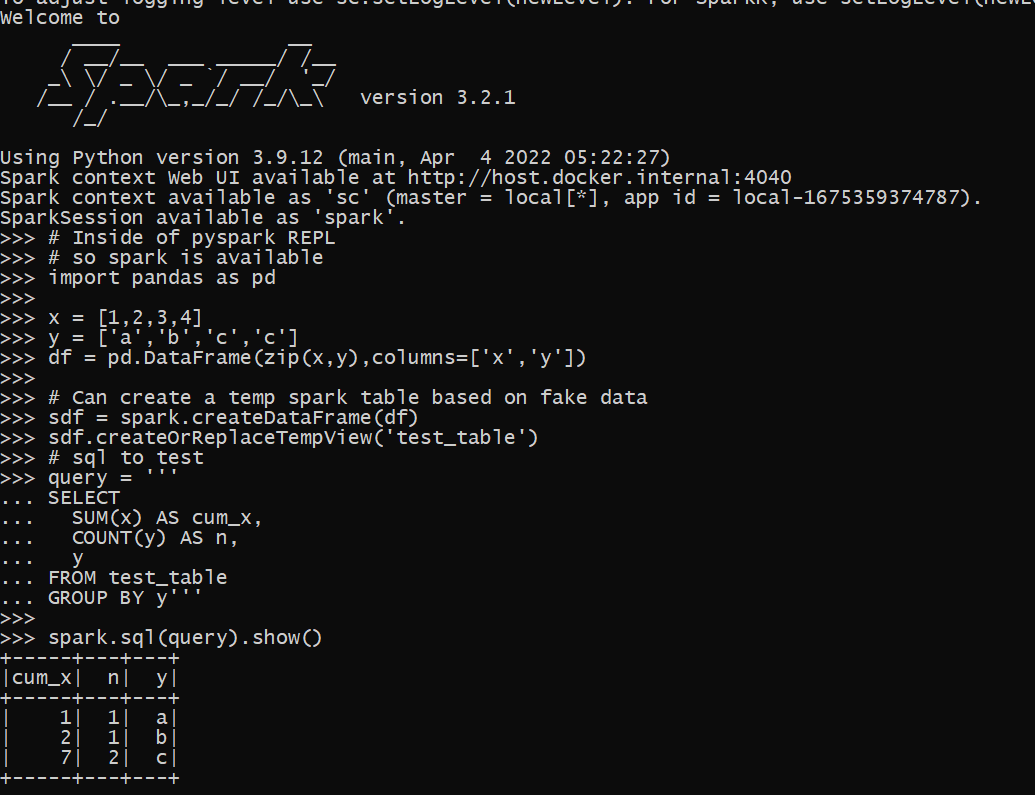
And voila, you can now test your spark queries. Although this is showing for spark, you can do something very similar for different databases as well, e.g. using pyodbc or sqlalchemy. You would want to have a test dummy database you can write to though to do that (a few different databases have volatile or temp tables equivalent to spark here).
Setting up pytest + spark
So this shows in just a REPL session how to set up this, but we also want automated tests for multiple scripts via pytest. To illustrate, I am going to refer to my retenmod repo. Even though this library obviously has nothing directly to do with pyspark, I am using this repo as a way to test code/python packaging. (And note if using the same environment above, to replicate 100% of that repo, need to install pip install black flake jupyter jupyter_contrib_nbextensions pre-commit matplotlib.)
So now for pytest, a special thing is you can create python objects that are inherited for all of your tests. Here we will create the spark object one time, and then it can be passed on to your tests. So in ./tests make a file conftest.py, and in this file write:
# This is inside of conftest.py
import pytest
from pyspark.sql import SparkSession

# This sets the spark object for the entire session
@pytest.fixture(scope="session")
def spark():
    sp = SparkSession.builder.getOrCreate()
    # Then can do other stuff to set
    # the spark object
    sp.sparkContext.setLogLevel("ERROR")
    sp.conf.set("spark.sql.execution.array.pyspark.enabled", "true")
    return sp
In pytest lingo, fixtures are then passed around to the different test functions in your library (where appropriate). You can create the equivalent of spark in a pyspark session via SparkSession.builder. This is essentially what a pyspark session is doing under the hood to generate the spark object you can run queries against.
Now we can make a test function, here in a file named test_spark.py (in the same tests folder). That will then look something like:
# pseudo code to show off test
# in test_spark.py
import pandas as pd
from yourlibrary import func

test_table = ...code to create dummy table...

def test_sql(spark):
    # Create the temporary table in spark
    sdf = spark.createDataFrame(test_table)
    sdf.createOrReplaceTempView("test_table")
    # Test out our sql query
    query = func(...your parameters to generate sql...)
    res = spark.sql(query).toPandas()
    # No guarantees on row order in this result
    # so I sort pandas dataframe to make 100% sure
    res.sort_values(by="y", inplace=True, ignore_index=True)
    # Then I do tests
    # Type like tests, shape and column names
    assert res.shape == (3, 3)
    assert list(res) == ["cum_x", "n", "y"]
    # Mathy type tests
    dif_x = res["x"] != [1, 2, 7]
    assert dif_x.sum() == 0
    dif_n = res["n"] != [1, 1, 2]
    assert dif_n.sum() == 0
So note here that I pass in spark as an argument to the function. pytest then uses the fixture we defined earlier to pass into the function when the test is actually run. And then from the command line you can run pytest to check out if your tests pass! (I have placed in the retenmod package a function to show off generating a discrete time survival table in spark, will need to do another blog post though on survival analysis using SQL.)
So this shows off what most of my sql type tests look like. I test that the shape of the data is how I expected (given my fake dataframe I passed in), columns are correct, and that the actual values are what they should be. I find this useful especially to test edge cases (such as missing data) in my SQL queries. My functions in production are mostly parameterized SQL, but it would work the same if you had a series of text SQL files, just read them into python as strings.
Setting up github actions
As a bonus, I show how to set this up in an automatic CICD check via github actions. Check out the actions workflow file for the entire workflow in-situ. But the YAML file has a few extra steps compared to my prior post on generating a wheel file in github actions.
It is short enough an can just paste the whole YAML file for you to check out.
on:
push:
branches:
- main
jobs:
build_wheel:
runs-on: ubuntu-latest
timeout-minutes: 20
steps:
- uses: actions/checkout@v2
- uses: actions/setup-java@v1
with:
java-version: 11
- uses: vemonet/setup-spark@v1
with:
spark-version: '3.2.1'
hadoop-version: '3.2'
- name: Set up Python
uses: actions/setup-python@v2
with:
python-version: 3.9
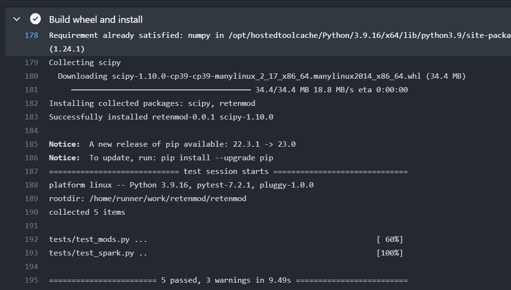
- name: Build wheel and install
run: |
python -m pip install --user --upgrade build
python -m build
# installing spark libraries
pip install pyspark pyarrow pandas pytest
# now install the wheel file
find ./dist/*.whl | xargs pip install
# Now run pytest tests
pytest --disable-warnings ./tests
- name: Configure Git
run: |
git config --global user.email "apwheele@gmail.com"
git config --global user.name "apwheele"
- name: Commit and push wheel
run: |
git add -f ./dist/*.whl
git commit -m 'pushing new wheel'
git push
- run: echo "🍏 This job's status is ${{ job.status }}."So here in addition to python, this also sets up Java and Spark. (I need to learn how to build actions myself, I wish vemonet/setup-spark@v1 had an option to cache the spark file instead of re-downloading everytime). Even with that though, it will only take a minute or two to run (the timeout is just a precaution and good idea to put in any github action).
You can then check this action out on github.
Happy SQL code testing for my fellow data scientists!