Reloading classes in python and shared borders

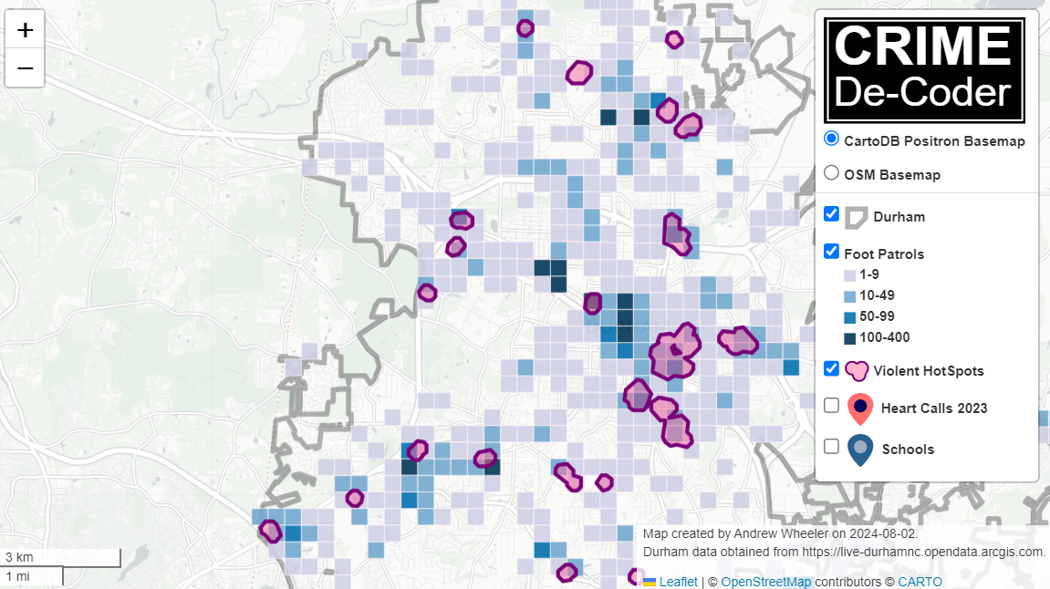
For some housekeeping, if you are not signed up, also make sure to sign up for the RSS feed of my crime de-coder blog. I have not been cross posting here consistently. For the last few posts:

For ASEBP, conference submissions for 2026 are open. (I will actually be going to this in 2026, submitted a 15 minute talk on planning experiments.)

Today will just be a quick post on two pieces of code I thought might be useful to share. The first is useful for humans, when testing code in functions, you can use the importlib library to reload functions. That is, imagine you have code:

import crimepy as cpy

test = cpy.func1(....)

And then when you run this, you see that func1 has an error. You can edit the source code, and then run:

from importlib import reload

reload(cpy)
test = cpy.func1(....)

This is my preferred approach to testing code. Note you need to import a library and reload the library. Not from crimepy import *, this will not work unfortunately.

Recently was testing out code that took quite a while to run, my Patrol Districting. This is a class, and I was editing my methods to make maps. The code itself takes around 5 minutes to run it through when remaking the entire class. What I found was a simpler approach, I can dump out the file to pickle, then reload the library, then load the pickle object. The may the pickle module works, it pulls the method definition from the global environment (pickle just saves the dict items under the hood). So the code looked like this:

from crimepy import pmed
...
pmed12 = pmed.pmed(...)
pmed12.map_plot() # causes error

And then instead of using the reload method as is (which would require me to create an entirely new object), use this approach for de-bugging:

# save file
import pickle
with open('pmed12.pkl', 'wb') as file:
    # Dump data with highest protocol for best performance
    pickle.dump(pmed12, file)

from importlib import reload
# edit method
reload(pmed)

# reload the object
with open('pmed12.pkl', 'rb') as file:
    # Load the pickled data
    pmed12_new = pickle.load(file)

# retest the method
pmed12_new.map_plot()

Writing code itself is often not the bottleneck – testing is. So figuring out ways to iterate testing faster is often worth the effort (I might have saved a day or two of work if I did this approach sooner when debugging that code).

The second code snippet is useful for the machines; I have been having Claude help me write quite a bit of the crimepy work. Here was one though it was having trouble with – calculating the shared border length between two polygons. Basically it went down an overly complicated path to get the exact calculation, whereas here I have an approximation using tiny buffers that works just fine and is much simpler.

def intersection_length(poly1,poly2,smb=1e-15):
    '''
    Length of the intersection between two shapely polygons
    
    poly1 - shapely polygon
    poly2 - shapely polygon
    smb - float, defaul 1e-15, small distance to buffer
    
    The way this works, I compute a very small buffer for
    whatever polygon is simpler (based on length)
    then take the intersection and divide by 2
    so not exact, but close enough for this work
    '''
    # buffer the less complicated edge of the two
    if poly1.length > poly2.length:
        p2, p1 = poly1, poly2
    else:
        p1, p2 = poly1, poly2
    # This basically returns a very skinny polygon
    pb = p1.buffer(smb,cap_style='flat').intersection(p2)
    if pb.is_empty:
        return 0.0
    elif hasattr(pb, 'length')
        return (pb.length-2*smb)/2
    else:
        return 0.0

And then for some tests:

from shapely.geometry import Polygon

poly1 = Polygon([(0, 0), (4, 0), (4, 3), (0, 3)])  # Rectangle
poly2 = Polygon([(2, 1), (6, 1), (6, 4), (2, 4)])  # Overlapping rectangle

intersection_length(poly1,poly2) # should be close to 0

poly3 = Polygon([(0, 0), (2, 0), (2, 2), (0, 2)])
poly4 = Polygon([(2, 0), (4, 0), (4, 2), (2, 2)])

intersection_length(poly3,poly4) # should be close to 2

poly5 = Polygon([(0, 0), (2, 0), (2, 2), (0, 2)])
poly6 = Polygon([(2, 0), (4, 0), (4, 3), (1, 3), (1, 2), (2, 2)])

intersection_length(poly5,poly6) # should be close to 3

poly7 = Polygon([(0, 0), (2, 0), (2, 2), (0, 2)])
poly8 = Polygon([(3, 0), (5, 0), (5, 2), (3, 2)])

intersection_length(poly7,poly8) # should be 0

Real GIS data often has imperfections (polygons that do not perfectly line up). So using the buffer method (and having an option to increase the buffer size) can often help smooth out those issues. It will not be exact, but the inexactness we are talking about will often be to well past the 10th decimal place.

Reducing folium map sizes

Recently for a crimede-coder project I have been building out a custom library to make nice leaflet maps using the python folium library. See the example I have posted on my website. Below is a screenshot:

This map ended up having around 3000 elements in it, and was a total of 8mb. 8mb is not crazy to put on a website, but is at the stage where you can actually notice latency when first rendering the map.

Looking at the rendered html code though it was verbose in a few ways for every element. One is that lat/lon are in crazy precision by default, e.g. [-78.83229390597961, 35.94592660794455]. So a single polygon can have many of those. Six digits of precision for lat/lon is still under 1 meter of precision, which is plenty sufficient for my mapping applications. So you can reduce 8+ characters per lat/lon and not really make a difference to the map (you can technically have invalid polygons doing this, but this is really pedantic and should be fine).

A second part of the rendered folium html map for every object is given a full uuid, e.g. geo_json_a19eff2648beb3d74760dc0ddb58a73d.addTo(feature_group_2e2c6295a3a1c7d4c8d57d001c782482);. This again is not necessary. I end up reducing the 32 length uuids to the first 8 alphanumeric characters.

A final part is that the javascript is not minified – it has quite a bit of extra lines/spaces that are not needed. So here are my notes on using python code to take care of some of those pieces.

To clean up the precision for geometry objects, I do something like this.

import re

# geo is the geopandas dataframe
redg = geo.geometry.set_precision(10**-6).to_json()
# redg still has floats, below regex clips values
rs = r'(\d{2}\.|-\d{2}\.)(\d{6})(\d+)'
re.sub(rs,r'\1\2',redg)

As most of my functions add the geojson objects to the map one at a time (for custom actions/colors), this is sufficient to deal with that step (for markers, can round lat/lon directly). It may make more sense for the set precision to be 10**-5 and then clip the regex. (For these regex’s I am showing there is some risk they will replace something they should not, I think it will be pretty safe though.)

Then to clean up the UUID’s and extra whitespace, what I do is render the final HTML and then use regex’s:

# fol is the folium object
html = fol.get_root()
res = html.script.get_root().render()
# replace UUID with first 8
ru = r'([0-9a-f]{8})[0-9a-f]{4}[0-9a-f]{4}[0-9a-f]{4}[0-9a-f]{12}'
res = re.sub(ru,r'\1',res)
# clean up whitespace
rl = []
for s in res.split('\n'):
    ss = s.strip()
    if len(ss) > 0:
        rl.append(ss)
rlc = '\n'.join(rl)

There is probably a smarter way to do this directly with the folium object for the UUID’s. For whitespace though it would need to be after the HTML is written. You want to be careful with the cleaning up the whitespace step – it is possible you wanted blank lines in say a leaflet popup or tooltip. But for my purposes this is not really necessary.

Doing these two steps in the Durham map reduces the size of the rendered HTML from 8mb to 4mb. So reduced the size of the file by around 4 million characters! The savings will be even higher for maps with more elements.

One last part is my map has redundant svg inserted for the map markers. I may be able to use css to insert the svg, e.g. something like in css .mysvg {background-image: url("vector.svg");}, and then in the python code for the marker svg insert <div class="mysvg"></div>. For dense point maps this will also save quite a few characters. Or you could add in javascript to insert the svg as well (although that would be a bit sluggish I think relative to the css approach, although sluggish after first render if the markers are turned off).

I have not done this yet, as I need to tinker with getting the background svg to look how I want, but could save another 200-300 characters per marker icon. So will save a megabyte in the map for every 3000-5000 markers I am guessing.

The main reason I post webdemo’s on the crimede-coder site is that there a quite a few grifters in the tech space. Not just for data analysis, but for front-end development as well. I post stuff like that so you can go and actually see the work I do and its quality. There are quite a few people now claiming to be “data viz experts” who just embed mediocre Tableau or PowerBI apps. These apps in particular tend to produce very bad maps, so here you can see what I think a good map should look like.

If you want to check out all the interactions in the map, I posted a YouTube video walking through them

Durham hotspot map walkthrough of interactions

GUI Tool to download Google Streetview Imagery

For some brief updates, check out the newest post on the CRIME De-Coder blog, PDs should share crime data. I discuss the types of crime data PDs typically share, the benefit to doing so, and how it can be very easy (just upload a static file to a website).

Also wanted to share a new tool I built, a GUI interface to download multiple Google Streetview images given a list of addresses. Here is a video of the tool in action:

I have been asked in the past to do this based on several blog posts I have written (1,2). I get around 200 views of those posts per month, so figured it was worth some time to build something general to share – it is often people in marketing interested in that data.

I am selling the tool for $300. Check out the CRIME De-Coder Store to purchase. It is currently built for Windows, I can build it for Mac if there is demand. (If you have a list and just want me to download the images for you, e.g. you don’t want to sign up for a google API key yourself, just get in touch and I will give a quote based on your total volume.)

If you are wondering where the $300 pricing came in, there is a simple rule that if you can estimate the maximum price someone is willing to buy, divide by half and that is reasonably close to optimal on typical sloping downward demand curves. I had an offer for $600 for this recently, hence I set the price of the tool for $300.

If there is other web-scraping data you are interested, always feel free to get in touch. I can often give quick feedback as to the feasibility and give a quote for the work (as well as detail if what you are asking is even feasible given the data available).

An alt take on opioid treatment coverage in North Carolina

The Raleigh News & Observer has been running multiple stories on the recent Medicaid expansion in North Carolina, with one recently about expanded opioid treatment coverage. Myself and Kaden Call have worked in the past on developing an algorithm to identify underprovided estimates (see background blog post, and Kaden’s work at Gainwell while an intern).

I figured I would run our algorithm through to see what North Carolina looks like. So here is an interactive map, with the top 10 zipcodes that have need for service (in red polygons), and CMS certified opioid treatment providers (in blue pins). (Below is a static image)

My initial impression was that this did not really jive with the quotes in the News & Observer article that suggested NC was a notorious service dessert – there are quite a few treatment providers across the state. So the cited Rural HealthInfo source disagrees with this. I cannot find their definition offhand, but I am assuming this is due to only counting in-patient treatment providers, whereas my list of CMS certified providers is mostly out-patient.

So although my algorithm identified various areas in the state that likely could use expanded services, this begs the question of whether NC is really a service dessert. It hinges on whether you think people need in-patient or out-patient treatment. Just a quick sampling of those providers, maybe half say they only take private, so it is possible (although not certain) that the recent Medicaid expansion will open up many treatment options to people who are dependent on opioids.

SAMHSA estimates that of those who get opioid treatment, around 5% get in-patient services. So maybe in the areas of high need I identify there is enough demand to justify opening new in-patient service centers – it is close though I am not sure the demand justifies opening more in-patient (as opposed to making it easier to access out-patient).

Asking folks with a medical background at work, it seems out-patient has proven to be as effective as in-patient, and that the biggest hurdle is to get people on buprenorphine/methadone/naltrexone (which the out-patient can do). So I am not as pessimistic as many of the health experts that are quoted in the News & Observer article.

Random notes, digital art, and pairwise comparisons is polynomial

So not too much in the hopper for the blog at the moment. Have just a bunch of half-baked ideas (random python tips, maybe some crime analysis using osmnx, scraping javascript apps using selenium, normal nerd data science stuff).

Still continuing my blog series on the American Society of Evidence Based Policing, and will have a new post out next week on officer use of force.

If you have any suggestions for topics always feel free to ask me anything!


Working on some random digital art (somewhat focused on maps but not entirely). For other random suggestions I like OptArt and Rick Wicklin’s posts.

Dall-E is impressive, and since it has an explicit goal of creating artwork I think it is a neat idea. Chat bots I have nothing good to say. Computer scientists working on them seem to be under the impression that if you build a large/good enough language model out pops general intelligence. Wee bit skeptical of that.


At work a co-worker was working on timing applications for a particular graph-database/edge-detection project. Initial timings on fake data were not looking so good. Here we have number of nodes and timings for the application:

  Nodes    Minutes
   1000       0.16
  10000       0.25
 100000       1.5
1000000      51

Offhand people often speak about exponential functions (or growth), but here what I expect is we are really looking at is pairwise comparisons (not totally familiar with the tech the other data scientist is using, so I am guessing the algorithmic complexity). So this likely scales something like (where n is the number of nodes in the graph):

Time = Fixed + C1*(n) + C2*(n choose 2) + e

Fixed is just a small constant, C1 is setting up the initial node database, and C2 is the edge detection which I am guessing uses pairwise comparisons, (n choose 2). We can rewrite this to show that the binomial coefficient is really polynomial time (not exponential) in terms of just the number of nodes.

C2*[n choose 2] = C2*[{n*(n-1)}/2]
                  C2*[ (n^2 - n)/2 ]
                  C2/2*[n^2 - n]
                  C2/2*n^2 - C2/2*n

And so we can rewrite our original equation in terms of simply n:

Time = Fixed + (C1 - C2/2)*N + C2/2*N^2

Doing some simple R code, we can estimate our equation:

n <- 10^(3:6)
m <- c(0.16,0.25,1.5,51)
poly_mod <- lm(m ~ n + I(n^2))

Since this fits 3 parameters with only 4 observations, the fit is (not surprisingly) quite good. Which to be clear does not mean much, if really cared would do much more sampling (or read the docs more closely about the underlying tech involved):

> pred <- predict(poly_mod)
> cbind(n,m,pred)
      n     m       pred
1 1e+03  0.16  0.1608911
2 1e+04  0.25  0.2490109
3 1e+05  1.50  1.5000989
4 1e+06 51.00 50.9999991

And if you do instead poly_2 <- lm(m ~ n + choose(n,2)) you get a change in scale of the coefficients, but the same predictions.

We really need this to scale in our application at work to maybe over 100 million records, so what would we predict in terms of minutes based on these initial timings?

> nd = data.frame(n=10^(7:8))
> predict(poly_mod,nd)/60 # convert to hours
         1          2
  70.74835 6934.56850

So doing 10 million records will take a few days, and doing 100 million will be close to 300 days.

With only 4 observations not much to chew over (really it is too few to say it should be a different model). I am wondering though how to best handle errors for these types of extrapolations. Errors are probably not homoskedastic for such timing models (error will be larger for larger number of nodes). Maybe better to use quantile regression (and model the median?). I am not sure (and that advice I think will also apply to modeling exponential growth as well).

Preprint: Analysis of LED street light conversions on firearm crimes in Dallas, Texas

I have a new pre-print out, Analysis of LED street light conversions on firearm crimes in Dallas, Texas. This work was conducted in collaboration with the Child Poverty Action Lab, in reference to the Dallas Taskforce report. Instead of installing the new lights though at hotspots that CPAL suggested, Dallas stepped up conversion of street lamps to LED. Here is the temporal number of conversions over time:

And here is an aggregated quadrat map at quarter square mile grid cells (of the total number of LED conversions):

I use a diff-in-diff design (compare firearm crimes in daytime vs nighttime) to test whether the cumulative LED conversions led to reduced firearm crimes at nighttime. Overall I don’t find any compelling evidence that firearm crimes were reduced post LED installs (for a single effect or looking at spatial heterogeneity). This graph shows in the aggregate the DiD parallel trends assumption holds citywide (on the log scale), but the identification strategy really relies on the DiD assumption within each grid cell (any good advice for graphically showing that with noisy low count data for many units I am all ears!).

For now just wanted to share the pre-print. To publish in peer-review I would need to do a bunch more work to get the lit review where most CJ reviewers would want it. Also want to work on spatial covariance adjustments (similar to here, but for GLM models). Have some R code started for that, but needs much more work/testing before ready for primetime. (Although as I say in the pre-print, these should just make standard errors larger, they won’t impact the point estimates.)

So no guarantees that will be done in anytime in the near future. But no reason to not share the pre-print in the meantime.

Getting census data over time

A former student recently asked about getting census data over time, in particular for smaller geographies like block groups. My GIS course I teach students the manual way of downloading data year-by-year from the FTP site. That is partially for pedagogical reasons though, I want students to realize the number of variables (there are so many) and how the data is stored by the census for the American Community Survey.

But Census now has a web api, where you can query the data. So if you are familiar with R or python programming, you can get the data in a bit easier fashion. You just need to know the years + census geographies + variables. I have notes on variables I often use for crim research, but going to the FTP site you can find the big documents or the excel templates.

I have honestly avoided these APIs in my workflows for several years, as my experience with the Census geocoding API was quite flaky, but I have not had the same problems with the APIs for querying the data. Here are examples in R (tidycensus library) and python (census library) of downloading several variables over the 2014-2019 span.

#############################
# R code
library(tidycensus)

# sign up for census key#
# https://api.census.gov/data/key_signup.html
census_api_key(key='????yourkeyhere????')

# place to store results and combine them
years <- 2014:2019
res <- vector("list",length(years))
names(res) <- years

# variables that you want
#        Tot Pop     White non-Hisp  FemHeadHouse  FamPoverty
vars <- c('B03001_001','B03002_003','B11003_016','B17010_002')

# loop over years, save data
# could also apply county filter, see help(get_acs)
# using smaller Deleware just for example
for (y in years){
    # download data
    ld <- as.data.frame(get_acs(year = y,
                                geography='cbg',
                                survey='acs5',
                                variables = vars,
                                state="DE"))
    # reshape long to wide
    ld2 <- reshape(ld,
                   idvar="GEOID",
                   timevar="variable",
                   direction="wide",
                   drop=c("NAME","moe"))
    # insert into list and add in year
    res[[y]] <- ld2
    res[[y]]$year <- y
}

# Combining the data frames together for final analysis
combo <- do.call("rbind",res)
head(combo) # can see B03001_001 is missing for block groups
summary(combo)
#############################

So in R you can ask for a variable, but if it is not available you will just get missing. So you need to make sure the variables you ask for are available over the time span.

The python census library will just straight up give you an error if the variable is not available. Also you need to specify E/M estimates, not just the base variable.

#############################
# Python code

from census import Census
import pandas as pd

key = '????yourkeyhere????'
c = Census(key)
# will get error with unknown variable
# need to specify E/M for estimate or margin of error
vars = ['B03002_003E','B11003_016E','B17010_002E']
res = []

for y in range(2014,2019+1):
    # '10' is Delaware, first '*' is county, second '*' is specific
    # geoid for a block group
    lk = c.acs5.state_county_blockgroup(vars, '10', "*", "*",year=y)
    ld = pd.DataFrame(lk)
    ld['year'] = y
    res.append(ld)

combo = pd.concat(res,axis=0)
combo.head()
#############################

(Initial post had an error not passing in year into the download function, now the two results are the same.)

For making reproducible scripts, instead of putting your API key into the code, a common way is to create a config file with the API key (don’t upload the config file to github), and then read in the config file into your script. (Another way is to use environment variables as secrets, I think the config is easier for people to grok though.)

Another friend recently referred me to requests-cache library. It is a good idea to only download the data locally once, then use that local data. No need to requery the data every time you update your code. Easiest approach is to just have a special script to download the data and save it (in a database or csv files would work here), and then later scripts work with that local data.

Downloading Social Vulnerability Index data

So Gainwell has let me open source one of the projects I have been working on at work – a python package to download SVI data. The SVI is an index created by the CDC to identify areas of high health risk in four domains based on census data (from the American Community Survey).

For my criminologist friends, these are very similar variables we typically use to measure social disorganization (see Wheeler et al., 2018 for one example criminology use case). It is a simple python install, pip install svi-data. And then you can get to work. Here is a simple example downloading zip code data for the entire US.

import numpy as np
import pandas as pd
import svi_data

# Need to sign up for your own key
key = svi_data.get_key('census_api.txt')

# Download the data from census API
svi_zips = svi_data.get_svi(key,'zip',2019)
svi_zips['zipcode'] = svi_zips['GEO_ID'].str[-5:]

Note I deviate from the CDC definition in a few ways. One is that when I create the themes, instead of using percentile rankings, I z-score the variables instead. It will likely result in very similar correlations, but this is somewhat more generalizable across different samples. (I also change the denominator for single parent heads of households to number of families instead of number of households, I think that is likely just an error on CDC’s part.)

Summed Index vs PCA

So here quick, lets check out my z-score approach versus a factor analytic approach via PCA. Here I just focus on the poverty theme:

pov_vars = ['EP_POV','EP_UNEMP','EP_PCI','EP_NOHSDP','RPL_THEME1']
svi_pov = svi_zips[['zipcode'] + pov_vars ].copy()

from sklearn import decomposition
from sklearn.preprocessing import scale

svi_pov.corr()

Note the per capita income has a negative correlation, but you can see the index works as expected – lower correlations for each individual item, but fairly high correlation with the summed index.

Lets see what the index would look like if we used PCA instead:

pca = decomposition.PCA()
sd = scale(svi_pov[pov_vars[:-1]])
pc = pca.fit_transform(sd)
svi_pov['PC1'] = pc[:,0]
svi_pov.corr() #almost perfect correlation

You can see that besides the negative value, we have an almost perfect correlation between the first principal component vs the simpler sum score.

One benefit of PCA though is a bit more of a structured approach to understand the resulting indices. So we can see via the Eigen values that the first PC only explains about 50% of the variance.

print(pca.explained_variance_ratio_)

And if we look at the loadings, we can see a more complicated pattern of residual loadings for each sucessive factor.

comps = pca.components_.T
cols = ['PC' + str(i+1) for i in range(comps.shape[0])]
load_dat = pd.DataFrame(comps,columns=cols,index=pov_vars[:-1])
print(load_dat)

So for PC3 for example, it has areas with high no highschool, as well as high per capita income. So higher level components can potentially identify more weird scenarios, which healthcare providers probably don’t care about so much by is a useful thing to know for exploratory data analysis.

Mapping

Since these are via census geographies, we can of course map them. (Here I grab zipcodes, but the code can download counties or census tracts as well.)

We can download the census geo data directly into geopandas dataframe. Here I download the zip code tabulation areas, grab the outline of Raleigh, and then only plot zips that intersect with Raleigh.

import geopandas as gpd
import matplotlib.pyplot as plt

# Getting the spatial zipcode tabulation areas
zip_url = r'https://www2.census.gov/geo/tiger/TIGER2019/ZCTA5/tl_2019_us_zcta510.zip'
zip_geo = gpd.read_file(zip_url)
zip_geo.rename(columns={'GEOID10':'zipcode'},inplace=True)

# Merging in the SVI data
zg = zip_geo.merge(svi_pov,on='zipcode')

# Getting outline for Raleigh
ncp_url = r'https://www2.census.gov/geo/tiger/TIGER2019/PLACE/tl_2019_37_place.zip'
ncp_geo = gpd.read_file(ncp_url)
ral = ncp_geo[ncp_geo['NAME'] == 'Raleigh'].copy()
ral_proj = 'EPSG:2278'
ral_bord = ral.to_crs(ral_proj)

ral_zips = gpd.sjoin(zg,ral,how='left')
ral_zips = ral_zips[~ral_zips['index_right'].isna()].copy()
ral_zipprof = ral_zips.to_crs(ral_proj)

# Making a nice geopandas static map, zoomed into Raleigh

fig, ax = plt.subplots(figsize=(6,6), dpi=100)

# Raleighs boundary is crazy
#ral_bord.boundary.plot(color='k', linewidth=1, edgecolor='k', ax=ax, label='Raleigh')
ral_zipprof.plot(column='RPL_THEME1', cmap='PRGn',
                 legend=True,
                 edgecolor='grey',
                 ax=ax)

# via https://stackoverflow.com/a/42214156/604456
ral_zipprof.apply(lambda x: ax.annotate(text=x['zipcode'], xy=x.geometry.centroid.coords[0], ha='center'), axis=1)

ax.get_xaxis().set_ticks([])
ax.get_yaxis().set_ticks([])

plt.show()

I prefer to use smaller geographies when possible, so I think zipcodes are about the largest areas that are reasonable to use this for (although I do have the ability to download this for counties). Zipcodes since they don’t nicely overlap city boundaries can cause particular issues in data analysis as well (Grubesic, 2008).

Other Stuff

I have a notebook in the github repo showing how to grab census tracts, as well as how to modify the exact variables you can download.

It does allow you to specify a year as well (in the notebook I show you can do the 2018 SVI for the 16/17/18/19 data at least). Offhand for these small geographies I would only expect small changes over time (see Miles et al., 2016 for an example looking at SES).

One of the things I think has more value added (and hopefully can get some time to do more on this at Gainwell), is to peg these metrics to actual health outcomes – so instead of making an index for SES, look at micro level demographics for health outcomes, and then post-stratify based on census data to get estimates across the US. But that being said, the SVI often does have reasonable correlations to actual geospatial health outcomes, see Learnihan et al. (2022) for one example that medication adherence the SVI is a better predictor than distance for pharmacy for example.

References

Use circles instead of choropleth for MSAs

We are homeschooling the kiddo at the moment (the plunge was reading by Bryan Caplan’s approach, and seeing with online schooling just how poor middle school education was). Wife is going through AP biology at the moment, and we looked up various job info on biomedical careers. Subsequently came across this gem of a map of MSA estimates from the Bureau of Labor Stats (BLS) Occupational Employment and Wage Stats series (OES).

I was actually mapping some metro stat areas (MSAs) at work the other day, and these are just terrifically bad geo areas to show via a choropleth map. All choropleth maps have the issue of varying size areas, but I never realized having somewhat regular borders (more straight lines) makes the state and county maps not so bad – these MSA areas though are tough to look at. (Wife says it scintillates for her if she looks too closely.)

There are various incredibly tiny MSAs next to giant ones that you will just never see in these maps (no matter what color scheme you use). Nevada confused for me quite a bit, until I zoomed in to see that there are 4 areas, Reno is just a tiny squib.

Another example is Boulder above Denver. (Look closely at the BLS map I linked, you can just make out Boulder if you squint, but I cannot tell what color it corresponds to in the legend.) The outline heavy OES maps, which are mostly missing data, are just hopeless to display like this effectively. Reno could be the hottest market for whatever job, and it will always be lost in this map if you show employment via the choropleth approach. So of course I spent the weekend hacking together some maps in python and folium.

The BLS has a public API, but I was not able to find the OES stats in that. But if you go through the motions of querying the data and muck around in the source code for those queries, you can see they have an undocumented API call to generate json to fill the tables. Then using this tool to convert the json calls to python (thank you Hacker News), I was able to get those tables into python.

I have these functions saved on github, so check out that source for the nitty gritty. But just here quickly, here is a replicated choropleth map, showing the total employees for bio jobs (you can go to here to look up the codes, or run my function bls_maps.ocodes() to get a pandas dataframe of those fields).

# Creating example bls maps
from bls_geo import *

# can check out https://www.bls.gov/oes/current/oes_stru.htm
bio = '172031'
bio_stats = oes_geo(bio)
areas = get_areas() # this takes a few minutes
state = state_albers()
geo_bio = merge_occgeo(bio_stats,areas)

ax = geo_bio.plot(column='Employment',cmap='inferno',legend=True,zorder=2)
state.boundary.plot(ax=ax,color='grey',linewidth=0.5,zorder=1)
ax.set_ylim(0.1*1e6,3.3*1e6)
ax.set_xlim(-0.3*1e7,0.3*1e7)   # lower 48 focus (for Albers proj)
ax.set_axis_off()
plt.show()

And that is not much better than BLSs version. For this data, if you are just interested in looking up or seeing the top metro areas, just doing a table, e.g. above geo_bio.to_excel('biojobs.xlsx'), works just as well as a map.

So I was surprised to see Minneapolis pop up at the top of that list (and also surprised Raleigh doesn’t make the list at all, but Durham has a few jobs). But if you insist on seeing spatial trends, I prefer to go the approach of mapping proportion or graduate circles, placing the points at the centroid of the MSA:

att = ['areaName','Employment','Location Quotient','Employment per 1,000 jobs','Annual mean wage']
form = ['',',.0f','.2f','.2f',',.0f']

map_bio = fol_map(geo_bio,'Employment',['lat', 'lon'],att,form)
#map_bio.save('biomap.html')
map_bio #if in jupyter can render like this

I am too lazy to make a legend, you can check out nbviewer to see an interactive Folium map, which I have tool tips (similar to the hover for the BLS maps).

Forgive my CSS/HTML skills, not sure how to make nicer popups. So you lose the exact areas these MSA cover in this approach, but I really only expect a general sense from these maps anyway.

These functions are general enough for whatever wage series you want (although these functions will likely break when the 2021 data comes out). So here is the OES table for data science jobs:

I feel going for the 90th percentile (mapping that to the 10 times programmer) is a bit too over the top. But I can see myself reasonably justifying 75th percentile. (Unfortunately these agg tables don’t have a way to adjust for years of experience, if you know of a BLS micro product I could do that with let me know!). So you can see here the somewhat inflated salaries for the SanFran Bay area, but not as inflated as many might have you think (and to be clear, these are for 2020 survey estimates).

If we look at map of data science jobs, varying the circles by that 75th annual wage percentile, it looks quite uniform. What happens is we have some real low outliers (wages under 70k), resulting in tiny circles (such as Athen’s GA). Most of the other metro regions though are well over 100k.

In more somber news, those interactive maps are built using Leaflet as the backend, which was create by a Ukranian citizen, Vladimir Agafonkin. We can do amazing things with open source code, but we should always remember it is on the backs of someones labor we are able to do those things.

Downloading geo files from Census FTP using python

I was working with some health data that only has MSA identifiers the other day. Not many people seem to know about the US Census’s FTP data site. Over the years they have had various terrible GUI’s to download data, but I almost always just go to the FTP site directly.

For geo data, check out https://www2.census.gov/geo/tiger/TIGER2019/ for example. Python for pandas/geopandas also has the nicety that you can point to a url (even a url of a zip file), and load in the data in memory. So to get the MSA areas was very simple:

# Example download MSA
import geopandas as gpd
from matplotlib import pyplot as plt

url_msa = r'https://www2.census.gov/geo/tiger/TIGER2019/CBSA/tl_2019_us_cbsa.zip'
msa = gpd.read_file(url_msa)
msa.plot()
plt.show()

Sometimes the census has files spread across multiple states. So here is an example of doing some simple scraping to get all of the census tracts in the US. You can combine the geopandas dataframes the same as pandas dataframes using pd.concat:

# Example scraping all of the zip urls on a page
from bs4 import BeautifulSoup
import pandas as pd
import re
import requests

def get_zip(url):
    front_page = requests.get(url,verify=False)
    soup = BeautifulSoup(front_page.content,'html.parser')
    zf = soup.find_all("a",href=re.compile(r"zip"))
    # Maybe should use href 
    zl = [os.path.join(url,i['href']) for i in zf]
    return zl

base_url = r'https://www2.census.gov/geo/tiger/TIGER2019/TRACT/'
res = get_zip(base_url)

geo_tract = []
for surl in res:
    geo_tract.append(gpd.read_file(surl))

geo_full = pd.concat(geo_tract)

# See State FIPS codes
# https://www.nrcs.usda.gov/wps/portal/nrcs/detail/?cid=nrcs143_013696

geo_full[geo_full['STATEFP'] == '01'].plot()
plt.show()

Unfortunately for the census data tables, such as https://www2.census.gov/programs-surveys/acs/summary_file/2019/data/5_year_seq_by_state/Alabama/Tracts_Block_Groups_Only/, those zip files contain two files (an estimate file and a margin of error file), so you cannot just do pd.read_csv(url) for those tables. But for the shapefile zip files this appears to work just fine and dandy.

I am currently working on a project at work (but Gainwell has given me the thumbs up to open source it) to build tables to create the CDC’s Social Vulnerability Index, which I can build for multiple geographies in combo with the census data. So hopefully in the next few weeks will be able to share that work.