Using docker to play with postgres

No major end of year updates. Life is boring (in a good way). My data science gig at Gainwell is going well. Still on occasion do scholarly type things (see my series on the American Society of Evidence Based Policing). Blog is still going strong, topping over 130k views this year.

As always, feel free to send me question, will just continue to post random tips over time related to things I am working on.


Post today is about using docker to run a personal postgres database. In the past I have attempted to install postgres on my personal windows machine, and this caused issues with other tool sets (in particular GIS tools that I believe rely on PostGIS somewhere under the hood). So a way around that is to install postgres on its entirely own isolated part of your machine. Using docker you don’t have to worry about messing things up – you can always just destroy the image you build and start fresh.

For background to follow along, you need to 1) install docker desktop on your machine, 2) have a python installation with in addition to the typical scientific stack sqlalchemy and psycopg2 (sqlalchemy may by default be installed on Anaconda distributions, I don’t think pyscopg2 is though).

For those not familiar, docker is a technology that lets you create virtual machines with certain specifications, e.g. something like “build an Ubuntu image with python and postgres installed”. Then you can do more complicated things, in data science we often are either creating an application server, or running batch jobs in such isolated environments. Here we will persist an image with postgres to test it out. (Both understanding docker and learning to work with databases and SQL are skills I expect more advanced data scientists to know.)

So first, again after you have docker installed, you can run something like:

docker run --name test_pg -p 5433:5432 -e POSTGRES_PASSWORD=mypass -d postgres

To create a default docker image that has postgres installed. This just pulls the base image postgres. Now you can get inside of that image, and add a schema/tables if you want:

docker exec -it test_pg bash
psql -U postgres
CREATE SCHEMA ts;
CREATE TABLE ts.test_tab (id serial primary key, val int, task text);
INSERT INTO ts.test_tab (val,task) values (1,'abc'), (2, 'def');
SELECT * FROM ts.test_tab;
\q

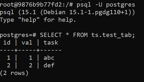
And you can do more complicated things, like install python and the postgres python extension.

# while still inside the postgres docker image
apt-get update
apt install python3 pip
apt-get install postgresql-plpython3-15
psql -U postgres
CREATE EXTENSION plpython3u;
\q
# head back out of image entirely
exit

(You could create a dockerfile to do all of this as well, but just showing step by step interactive here as a start. I recommend that link as a getting feet wet with docker as well.)

Now, back on your local machine, we can also interact with that same postgres database. Using python code:

import pandas as pd
import sqlalchemy
import psycopg2
import pickle

uid = 'postgres' # in real life, read these in as secrets
pwd = 'mypass'   # or via config files
ip = 'localhost:5433' # port is set on docker command

# depending on sqlalchemy version, it may be
# 'postgres' insteal of 'postgresql'
conn_str = f'postgresql://{uid}:{pwd}@{ip}/postgres'
eng = sqlalchemy.create_engine(conn_str)

res = pd.read_sql('SELECT * FROM ts.test_tab',eng)
print(res)

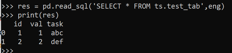
And you can save a table into this same database:

res['new'] = [True,False]
res.to_sql('new_tab',schema='ts',con=eng,index=False,if_exists='replace')
pd.read_sql('SELECT * FROM ts.new_tab',eng)

And like I said, I like to have a version I can test things with. One example, I have tested a deployment pattern that passes around binary blobs for model artifacts.

# Can save a python object as binary blob
eng.execute('''create table ts.mod (note VARCHAR(50) UNIQUE, mod bytea);''')

def save_mod(model, note, eng=eng):
    bm = pickle.dumps(model)
    md = psycopg2.Binary(bm)
    in_sql = f'''INSERT INTO ts.mod (note, mod) VALUES ('{note}',{md});'''
    info = eng.url # for some reason sqlalchemy doesn't work for this
    # but using psycopg2 directly does
    pcn = psycopg2.connect(user=info.username,password=info.password,
                          host=info.host,port=info.port,dbname=info.database)
    cur = pcn.cursor()
    cur.execute(in_sql)
    pcn.commit()
    pcn.close()

def load_mod(note, eng=eng):
    sel_sql = f'''SELECT mod FROM ts.mod WHERE note = '{note}';'''
    res = pd.read_sql(sel_sql,eng)
    mod = pickle.loads(res['mod'][0])
    return mod

This does not work out of the box for objects that have more complicated underlying code, but pure python stuff in sklearn it seems to work OK:

# Create random forest
import numpy as np
from sklearn.ensemble import RandomForestRegressor

train = np.array([[1,2],[3,4],[1,3]])
y = np.array([1,2,3])
mod = RandomForestRegressor(n_estimators=5,max_depth=2,random_state=0)
mod.fit(train,y)

save_mod(mod,'ModelRF1')
m2 = load_mod('ModelRF1')

# Showing the outputs are the same
mod.predict(train)
m2.predict(train)

You may say to yourself this is a crazy deployment pattern. And I would say I do what I need to do given the constraints I have sometimes! (I know more startups with big valuations that do SQL insertion to deploy models than ones with more sane deployment strategies. So I am not the only one.)

But this is really just playing around like I said. But you can try out more advanced stuff as well, such as using python inside postgres functions, or something like this postgres extension for ML models.

Startup scripts on windows

Just a very quick post today. For folks working on Unix machines, there is a bash profile script that runs when you first log into your user, and can set various environment variables, symlinks, or just run scripts in general. On windows, you can do something similar by placing program.bat files in the shell startup directory. (That linked post by Microsoft has the directions to find where that is located on your machine. Hit Windows Logo + R and type shell:startup into the prompt. It ends up being C:\Users\andre\AppData\Roaming\Microsoft\Windows\Start Menu\Programs\Startup on my personal machine.)

One I have is to map regular folders I use to particular drive letters (similar in outcomes to symlinks on Unix machines) using the subst command. So in that startup directory I have a file, ghub_map.bat, that contains this single line:

subst g: "D:\Dropbox\Dropbox\PublicCode_Git"

And so when I log into my machine, if I want to go and do work on github I can just do type G: in the windows terminal (to switch drives you don’t use cd in windows). This is in place of the more onerous, D: (default terminal starts in C:), and then cd ./Dropbox/Dropbox/PublicCode_Git.

Happy holidays everyone!

Handling errors in python and R

Just some quick notes on error handling in python and R. For most of my batch processes at work (in python), error handling is necessary. Most of my code has logic that if it fails, it sends an email message about the failure. This is only possible if you capture errors and have conditional logic, if the code just fails without capturing the error (for both R and python) it will just exit the script.

I had another example recently in R that used placebo tests that could fail to converge. So a more traditional stat project, but it should just keep running the loop to collect results, not fail entirely.

Python Example

In python, for most of my batch jobs I have code that looks like this:

import traceback

try:
    # whatever function you are running
    send_success_email()
except Exception:
    er = traceback.format_exc()
    print(f'Error message is \n\n{er}')
    send_error_email(er)

So it fails gracefully, and just gives me a message either in REPL for interactive debugging or stdout for regularly run batch jobs. I can see for people running servers why they want more specific error handling and using a more formal logger, but IMO that is overkill for running batch jobs.

R Example

R to do error handling looks something like this:

# trycatch for errors
my_func <- function(){
    # try/catch if error
    out <- tryCatch(
       { # part with the potential error
         #r <- ???? #whatever code steps you want
        r
       }, error=function(cond){ 
          print("Function Failed, Error message is \n\n")
          print(Cond)
          return(-1)
          } )
    return(out)
}

So if you have inside the tryCatch something that is “fit complicated model” inside your simulations (that could fail), this will still fail gracefully (and can return the error message if you need to.

Counting lines of code

Was asked recently about how many lines of python code was in my most recent project. A simple command line check, cd into your project directory and run:

find -type f -name "*.py" | xargs wc -l

(If on windows, you can download the GOW tools to be able to use these same tools by default available on unix/mac.) This will include whitespace and non-functional lines (like docstrings), but that I think is ok. Doing this for my current main project at Gainwell, I have about 30k lines of python code. Myself (and now about 4 other people) have been working on that code base for nearly a year.

For my first production project at (then) HMS, the total lines of python code are 20k, and I developed the bulk of that in around 7 months of work. Assuming 20 work days in a month, that results in around 20000/140 ~ 143 lines of code per workday. I did other projects during that time span, but this was definitely my main focus (and I was the sole developer/data scientist). I think that is high (more code is not necessarily better, overall code might have decreased as future development of this project happened over time), but is ballpark reasonable expectations for working data scientists (I would have guessed closer to around 100 per day). In the grand scheme of things, this is like 2 functions or unit tests per work day (when considering white space and docstrings).

Doing this for all of my python code on my personal machine is around 60k (I do around, as I am removing counts for projects that are just cloned). And for all the python code on my work machine is around 140k (for 3 years of work). (I am only giving fuzzy numbers, I have some projects joint work I am half counting, and some cloned code I am not counting at all.)

Doing this same exercise for R code, I only get around 40k lines of code on my personal machine. For instance, my ptools package has under 3k lines of "*.R" code total. I am guessing this is due to not only R code being more precise than python, but to take code into production takes more work. Maybe worth another blog post, but the gist of the difference between an academic project is that you need the code to run one time, whereas for a production project the code needs to keep running on a regular schedule indefinitely.

I have written much more SPSS code over my career than R code, but I have most of it archived on Dropbox, so cannot easily get a count of the lines. I have a total of 1846 sps files (note that this does not use xargs).

find -type f -name "*.sps" | wc -l

It is possible that the average sps file on my machine is 200 lines per file (it definitely is over 100 lines). So my recent python migration I don’t think has eclipsed my cumulative SPSS work going back over a decade (but maybe in two more years will).

Random notes, digital art, and pairwise comparisons is polynomial

So not too much in the hopper for the blog at the moment. Have just a bunch of half-baked ideas (random python tips, maybe some crime analysis using osmnx, scraping javascript apps using selenium, normal nerd data science stuff).

Still continuing my blog series on the American Society of Evidence Based Policing, and will have a new post out next week on officer use of force.

If you have any suggestions for topics always feel free to ask me anything!


Working on some random digital art (somewhat focused on maps but not entirely). For other random suggestions I like OptArt and Rick Wicklin’s posts.

Dall-E is impressive, and since it has an explicit goal of creating artwork I think it is a neat idea. Chat bots I have nothing good to say. Computer scientists working on them seem to be under the impression that if you build a large/good enough language model out pops general intelligence. Wee bit skeptical of that.


At work a co-worker was working on timing applications for a particular graph-database/edge-detection project. Initial timings on fake data were not looking so good. Here we have number of nodes and timings for the application:

  Nodes    Minutes
   1000       0.16
  10000       0.25
 100000       1.5
1000000      51

Offhand people often speak about exponential functions (or growth), but here what I expect is we are really looking at is pairwise comparisons (not totally familiar with the tech the other data scientist is using, so I am guessing the algorithmic complexity). So this likely scales something like (where n is the number of nodes in the graph):

Time = Fixed + C1*(n) + C2*(n choose 2) + e

Fixed is just a small constant, C1 is setting up the initial node database, and C2 is the edge detection which I am guessing uses pairwise comparisons, (n choose 2). We can rewrite this to show that the binomial coefficient is really polynomial time (not exponential) in terms of just the number of nodes.

C2*[n choose 2] = C2*[{n*(n-1)}/2]
                  C2*[ (n^2 - n)/2 ]
                  C2/2*[n^2 - n]
                  C2/2*n^2 - C2/2*n

And so we can rewrite our original equation in terms of simply n:

Time = Fixed + (C1 - C2/2)*N + C2/2*N^2

Doing some simple R code, we can estimate our equation:

n <- 10^(3:6)
m <- c(0.16,0.25,1.5,51)
poly_mod <- lm(m ~ n + I(n^2))

Since this fits 3 parameters with only 4 observations, the fit is (not surprisingly) quite good. Which to be clear does not mean much, if really cared would do much more sampling (or read the docs more closely about the underlying tech involved):

> pred <- predict(poly_mod)
> cbind(n,m,pred)
      n     m       pred
1 1e+03  0.16  0.1608911
2 1e+04  0.25  0.2490109
3 1e+05  1.50  1.5000989
4 1e+06 51.00 50.9999991

And if you do instead poly_2 <- lm(m ~ n + choose(n,2)) you get a change in scale of the coefficients, but the same predictions.

We really need this to scale in our application at work to maybe over 100 million records, so what would we predict in terms of minutes based on these initial timings?

> nd = data.frame(n=10^(7:8))
> predict(poly_mod,nd)/60 # convert to hours
         1          2
  70.74835 6934.56850

So doing 10 million records will take a few days, and doing 100 million will be close to 300 days.

With only 4 observations not much to chew over (really it is too few to say it should be a different model). I am wondering though how to best handle errors for these types of extrapolations. Errors are probably not homoskedastic for such timing models (error will be larger for larger number of nodes). Maybe better to use quantile regression (and model the median?). I am not sure (and that advice I think will also apply to modeling exponential growth as well).

Preprint: Analysis of LED street light conversions on firearm crimes in Dallas, Texas

I have a new pre-print out, Analysis of LED street light conversions on firearm crimes in Dallas, Texas. This work was conducted in collaboration with the Child Poverty Action Lab, in reference to the Dallas Taskforce report. Instead of installing the new lights though at hotspots that CPAL suggested, Dallas stepped up conversion of street lamps to LED. Here is the temporal number of conversions over time:

And here is an aggregated quadrat map at quarter square mile grid cells (of the total number of LED conversions):

I use a diff-in-diff design (compare firearm crimes in daytime vs nighttime) to test whether the cumulative LED conversions led to reduced firearm crimes at nighttime. Overall I don’t find any compelling evidence that firearm crimes were reduced post LED installs (for a single effect or looking at spatial heterogeneity). This graph shows in the aggregate the DiD parallel trends assumption holds citywide (on the log scale), but the identification strategy really relies on the DiD assumption within each grid cell (any good advice for graphically showing that with noisy low count data for many units I am all ears!).

For now just wanted to share the pre-print. To publish in peer-review I would need to do a bunch more work to get the lit review where most CJ reviewers would want it. Also want to work on spatial covariance adjustments (similar to here, but for GLM models). Have some R code started for that, but needs much more work/testing before ready for primetime. (Although as I say in the pre-print, these should just make standard errors larger, they won’t impact the point estimates.)

So no guarantees that will be done in anytime in the near future. But no reason to not share the pre-print in the meantime.

NIJ grants funding gun violence research

Before I get into the nitty gritty of this post, a few notes. First, my next post in the Criminal Justician series on ASEBP is up, Violent Crime Interventions That are Worth it. I discuss more of the costs with implementing hot spots policing and focussed deterrence from the police departments perspective, and why they are clearly worthwhile investments for many police departments facing violence problems.

Second, I want to point folks to Jacob Kaplan’s blog, most recent post The Covid Kings of Salami. Some of Jacob’s thoughts I disagree with (I think smaller papers are OK, or that policing what is big enough is a waste of time). But if you like my posts on CJ topics, you should check out Jacob’s as well.

Now onto the title – a work in progress at the moment, but working with Scott Jacques on the openness of funded US criminology research. A short post in response to the oft mistaken idea that gun violence research is banned in the US. This is confused logic related to the Dickey act saying awards for gun control advocacy are banned as being federally funded by the CDC.

There are other agencies who fund gun violence research, in particular here I have scraped data from the National Institute of Justice (what I think is likely to be the largest funder in this area). Here is some python code showing some analyses of those awards.

So first, here you can download and see the size of the scraped dataset of NIJ awards:

import pandas as pd

# award data scraped, stay tuned for code for that!
award_url = 'https://dl.dropbox.com/s/eon4iokv0qpllgl/NIJ_Awards.csv?dl=0'
award_df = pd.read_csv(award_url)
print(award_df.shape)
print(award_df['award_text'][0])

So as a first blush check for awards related to gun violence, we can just search the text for the award narrative for relevant terms, here I just search for GUN VIOLENCE and FIREARM. A more thorough investigation would either code the 7k awards or the original solicitations, but I think this will likely be largely accurate (probably slightly more false positives than false negatives).

award_df['award_textU'] = award_df['award_text'].str.upper()

# Lets try to find any of these (other text?)
word_list = ['GUN VIOLENCE','FIREARM']

for w in word_list:
    award_df[w] = 1*(award_df['award_textU'].str.find(w) > -1)

award_df['AnyGun'] = 1*(award_df[word_list].sum(axis=1) > 0)
print(award_df['AnyGun'].sum())

So we can see that we have 1,082 awards related to gun violence (out of 7,215 listed by the NIJ). Lets check out the total funding for these awards:

# Lets figure out the total allocated
award_df['AwardVal'] = award_df['field-award-amount'].str.strip()
award_df['AwardVal'] = award_df['AwardVal'].replace('[\$,]', '', regex=True)
award_df['AwardVal'] = pd.to_numeric(award_df['AwardVal'])
award_df['Tot'] = 1

cf = ['Tot','AwardVal']
award_df.groupby('AnyGun',as_index=False)[cf].sum()

So we have in the listed awards (that go back to 1998 but appear more consistently filled in starting in 2002), over 300 million in grant awards related to gun violence/firearm research. Here we can see the breakdown over time.

# See awards over time
gun_awards = award_df[award_df['AnyGun'] == 1].copy()
gun_awards.groupby('field-fiscal-year',as_index=False)[cf].sum()

So the awards gifted by NIJ no doubt have a different flavor/orientation than if you had the same money from CDC. (There are other orgs though, like NSF, who I am sure have funded research projects relevant to gun violence over time as well.) Sometimes people distinguish between “public health” vs “criminal justice” approaches, but this is a pretty superficial dichotomy (plenty of people in public health have gotten NIJ awards).

So you certainly could argue the Dickey amendment changed the nature of gun violence research being conducted. And since the CDC budget is so massive, I suppose you could argue that it reduced the overall amounts of gun violence research being funded (although it is likely 0 sum, more for firearm research would have slashed some other area). You could use the same argument to say NIJ though is underfunded instead of advocating for the CDC to write the checks though.

But the stronger statement I often see stated, that firearm research is entirely banned in the US, is not even close to being correct.

Injury rates at Amazon warehouses

I follow several of the News & Observer (The Raleigh/Durham newspaper) newsletters, and Brian Gordon and Tyler Dukes had a story recently about fainting and ambulance runs at the Amazon warehouse in Raleigh, Open Source: Ambulances at Amazon. He did some great sleuthing, and showed that while the number on its face seemed high (an ambulance call around 1 out of 3 days) the rate of ambulance runs when accounting for the size of the workforce is pretty similar to other warehouses.

Here I will show an example of downloading the OSHA injury data to show a similar finding. Using python it is pretty quick work.

So first can import the libraries we need (the typical scientific stack). I download the OSHA data for 2021, and I calculate injury rates per person work year, so how to interpret these are at the workplace level. Per full time people per year, it is the expected number of injuries across the workforce.

import pandas as pd
import matplotlib.pyplot as plt
import numpy as np
from scipy.stats import beta

inj_2021url = "https://www.osha.gov/sites/default/largefiles/ITA-data-cy2021.zip"
inj_dat = pd.read_csv(inj_2021url)
# Calculate injuries per person full year
inj_dat['InjPerYear'] = (inj_dat['total_injuries']/inj_dat['total_hours_worked'])*2080

We can filter out warehouse workers via NAICS code 493110. I also just limit to warehouses in North Carolina. Sorting by the injury rate, Amazon is not even in the top 10 in the state:

warehouses = inj_dat[inj_dat['naics_code'] == 493110].copy()
warehouses_nc = warehouses[warehouses['state'] == 'NC'].reset_index(drop=True)
warehouses_nc['AmazonFlag'] = 1*(warehouses_nc['company_name'].str.find('Amazon.com') >= 0)

# Rate per year of work per person, 2080 
warehouses_nc.sort_values('InjPerYear',ascending=False,ignore_index=True,inplace=True)
warehouses_nc.head(10)

But note that I don’t think Bonded Logistics is a terribly dangerous place. One thing you need to watch out for when evaluating rate data is that places with smaller denominators (here lower total hours worked) tend to be more volatile. So a useful plot is to plot the total hours work (cumulative for the entire warehouse) against the overall rate of injuries per hour worked.

fig, ax = plt.subplots(figsize=(12,6))
ax.scatter(nam_ware['total_hours_worked'], nam_ware['InjPerYear'], 
           c='grey', s=30, edgecolor='k', alpha=0.5, label='Other Warehouses')
ax.scatter(amz_ware['total_hours_worked'], amz_ware['InjPerYear'], 
           c='blue', s=80, edgecolor='k', alpha=0.9, label='Amazon Warehouses')
ax.set_axisbelow(True)
ax.set_xlabel('Total Warehouse Hours Worked')
ax.set_ylabel('Injury Rate per Person Work Year (2080 hours)')
ax.legend(loc='upper right')
plt.savefig('InjRate.png', dpi=500, bbox_inches='tight')

You can see by this plot the Amazon warehouses have the largest total number of hours worked (by quite a few) relative to many other warehouses in North Carolina. But their overall rate of injuries is right in line with the rest of the crowd. Looking at the overall rate, it is around 0.04 (so you would expect around 1/20 full time workers to have an injury per year at a warehouse according to this data).

tot_rate = warehouses_nc['total_injuries'].sum()/warehouses_nc['total_hours_worked'].sum()
print(tot_rate*2080)

If we do this plot again, but add funnel bound lines to show the typical volatility we would expect with estimating these rates:

# Binomial confidence interval
def binom_int(num,den,confint=0.95):
    quant = (1 - confint)/ 2.
    low = beta.ppf(quant, num, den - num + 1)
    high = beta.ppf(1 - quant, num + 1, den - num)
    return (np.nan_to_num(low), np.where(np.isnan(high), 1, high))

den = np.geomspace(1000,8700000,500)
num = den*tot_rate
low_int, high_int = binom_int(num,den,0.99)
high_int = high_int*2080

fig, ax = plt.subplots(figsize=(12,6))
ax.plot(den,high_int, c='k', linewidth=0.5)
ax.hlines(tot_rate*2080,1000,8700000,colors='k', linewidths=0.5)
ax.scatter(nam_ware['total_hours_worked'], nam_ware['InjPerYear'], 
           c='grey', s=30, edgecolor='k', alpha=0.5, label='Other Warehouses')
ax.scatter(amz_ware['total_hours_worked'], amz_ware['InjPerYear'], 
           c='blue', s=80, edgecolor='k', alpha=0.5, label='Amazon Warehouses')
ax.set_axisbelow(True)
ax.set_xlabel('Total Warehouse Hours Worked')
ax.set_ylabel('Injury Rate per Person Work Year (2080 hours)')
plt.xscale('log', basex=10)
ax.legend(loc='upper right')
ax.annotate('Straight line is average overall injury rate\nCurved line is Binomial 99% Interval', 
            xy = (0.00, -0.13), xycoords='axes fraction')
plt.savefig('InjRate_wBin.png', dpi=500, bbox_inches='tight')

So you can see even Bonded Logistics is well within the average rate you would expect to still be consistent with the average overall injury rate relative to all the other warehouses in North Carolina.

As a note, I imagine I saw someone using this data recently looking at police departments in a criminal justice paper (I have in my notes police departments are NAICS code 922120). (Maybe Justin Nix/Michael Sierra-Arévalo/Ian Adams?) But sorry do not remember the paper (so I owe credit to someone else for pointing out this data, but not sure who).

Another way to do the analysis is to calculate the lower/upper confidence intervals per the rates, and then sort by the lower confidence interval. This way you can filter out high rate variance locations.

# Can look at police departments
# NAICS code 922120
police = inj_dat[inj_dat['naics_code'] == 922120].copy()
low_police, high_police = binom_int(police['total_injuries'],police['total_hours_worked'])
police['low_rate'] = low_police*2080
police.sort_values('low_rate',ascending=False,ignore_index=True,inplace=True)
check_fields = ['establishment_name','city','state','total_injuries','total_hours_worked','InjPerYear','low_rate']
police[check_fields].head(10)

So you can see we have some funny business going on with the LA data reporting (which OSHA mentions on the data webpage). Maybe it is just admin duty, so people are already injured and get assigned to those bureaus (not sure why LAPD reports seperate bureaus at all).

New paper: An Open Source Replication of a Winning Recidivism Prediction Model

Our paper on the NIJ forecasting competition (Gio Circo is the first author), is now out online first in the International Journal of Offender Therapy and Comparative Criminology (Circo & Wheeler, 2022). (Eventually it will be in special issue on replications and open science organized by Chad Posick, Michael Rocque, and Eric Connolly.)

We ended up doing the same type of biasing as did Mohler and Porter (2022) to ensure fairness constraints. Essentially we biased results to say no one was high risk, and this resulted in “fair” predictions. With fairness constraints or penalities you sometimes have to be careful what you wish for. And because not enough students signed up, me and Gio had more winnings distributed to the fairness competition (although we did quite well in round 2 competition even with the biasing).

So while that paper is locked down, we have the NIJ tech paper on CrimRXiv, and our ugly code on github. But you can always email for a copy of the actual published paper as well.

Of course since not an academic anymore, I am not uber focused on potential future work. I would like to learn more about survival type machine learning forecasts and apply it to recidivism data (instead of doing discrete 1,2,3 year predictions). But my experience is the machine learning models need very large datasets, even the 20k rows here are on the fringe where regression are close to equivalent to non-linear and tree based models.

Another potential application is simple models. Cynthia Rudin has quite a bit of recent work on interpretable trees for this (e.g. Liu et al. 2022), and my linked post has examples for simple regression weights. I suspect the simple regression weights will work reasonably well for this data. Likely not well enough to place on the scoreboard of the competition, but well enough in practice they would be totally reasonable to swap out due to the simpler results (Wheeler et al., 2019).

But for this paper, the main takeaway me and Gio want to tell folks is to create a (good) model using open source data is totally within the capabilities of PhD criminal justice researchers and data scientists working for these state agencies.They are quantitaive skills I wish more students within our field would pursue, as it makes it easier for me to hire you as a data scientist!

References

Using IO objects in python to read data

Just a quick post on a technique I’ve used a few times recently, in particular when reading web data.

First for a very quick example, in python when reading data with pandas, it often expects a filename on disk. For pandas, e.g. pd.read_csv('my_file.csv'). But if you happen to already have the contents of the csv in a text object in memory, you can use io.StringIO to just read that object.

import pandas as pd
from io import StringIO

# Example csv file inline
examp_csv = """a,b
1,x
2,z"""

pd.read_csv(StringIO(examp_csv))

Where this has come up for me recently is reading in different data from web servers. For example, here is Cary’s API for crime data, you can batch download the whole thing at the below url, but via this approach I currently get an SSL error:

# Town of Cary CSV for crimes
cary_url = 'https://data.townofcary.org/explore/dataset/cpd-incidents/download/?format=csv&timezone=America/New_York&lang=en&use_labels_for_header=true&csv_separator=%2C'

# Returns SSL Error for me
cary_df = pd.read_csv(cary_url)

Note I don’t know the distinction in web server tech that causes this (as sometimes you can just grab a CSV via url, here is an example I have grabbing PPP loan data or with the NIJ recidivism data).

But we can grab the data via requests, and use the same StringIO trick I just showed to get this data:

# Using string IO for reading text
import requests
res_cary = requests.get(cary_url)
cary_df = pd.read_csv(StringIO(res_cary.text))
cary_df

Again I don’t know why some servers you need to go through this approach, but this works for me for Socrata and CartoDB api’s for different cities open data. I also used in recently for converting geojson in ESRI’s api.

The second example I want to show is downloading zipfiles. For this, we will use io.BytesIO instead of StringIO. The census stores various data in zipfiles on their FTP server:

# Example 2, grabbing zipped contents
import zipfile
from io import BytesIO

census_url = 'https://www2.census.gov/programs-surveys/acs/summary_file/2019/data/2019_5yr_Summary_FileTemplates.zip'
req = requests.get(census_url)

# Can use BytesIO for this content
zf = zipfile.ZipFile(BytesIO(req.content))

The zipfile library would be equivalent to reading/extracting a zipfile already on disk. But when downloading there is no need to save to disk, then deal with that file. BytesIO here cuts out the middleman.

Then we gan either grab a specific file inside of our zf object, or extract all the contents one-by-one:

# Now can loop through the list
# or grab specific file
zf.filelist[0]
temp_geo = pd.read_excel(zf.open('2019_SFGeoFileTemplate.xlsx'))
temp_geo.T