Neighborhoods in Albany according to Google

One of the most vexing aspects of spatial analysis in the social sciences in the concept of neighborhoods. There is a large literature on neighborhood effects in criminology, but no one can really define a neighborhood. For analysis they are most often assumed to approximately conform to census areas (like tracts or blocks). Sometimes there are obvious physical features that divide neighborhoods (most often a major roadway), but more often boundaries are fuzzy.

I’ve worked on several surveys (at the Finn Institute) in which we ask people what neighborhood they live in as well as the nearest intersection to their home. Even where there is a clear border, often people say the “wrong” neighborhood, especially near the borders. IIRC, when I calculated the wrongness for one survey in Syracuse we did it was only around 60% of the time the respondents stated they lived the right neighborhood. I do scare quotes around “wrong” because it is obviously arbitrary where people draw the boundaries, so more people saying the wrong neighborhood is indicative of the borders being misaligned than the respondents being wrong.

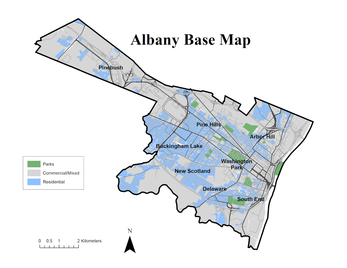
For this reason I like the Google maps approach in which they just place a label at the approximate center of noteworthy neighborhoods. I emulated this for a recent background map I made for a paper in Albany. (Maps can be opened in a separate tab to see a larger image.)

As background I did not grow up in Albany, but I’ve lived and worked in the Capital District since I came up to Albany for grad school – since 2008. Considering this and the fact that I make maps of Albany on a regular basis is my defense I have a reasonable background to make such judgements.

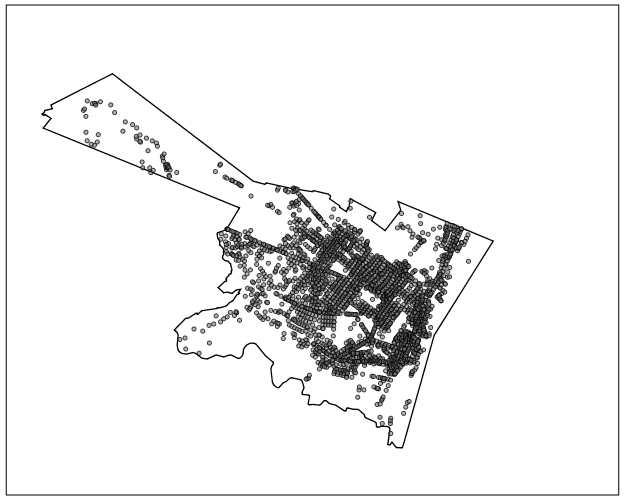
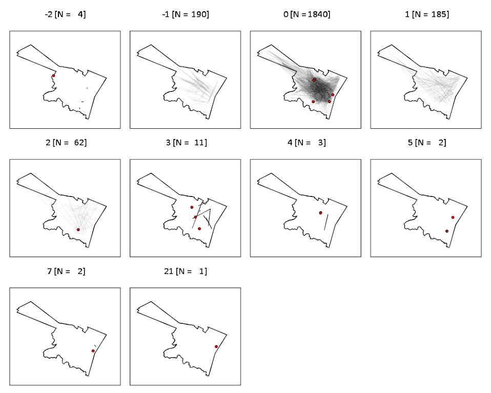
When looking at Google’s reverse geocoding API the other day I noticed they returned a neighborhood field in the response. So I created a regular sampling grid over Albany to see what they return. First, lets see my grid and where Google actually decides some neighborhood exists. Large grey circles are null, and small red circles some neighborhood label was returned. I have no idea where Google culls such neighborhood labels from.

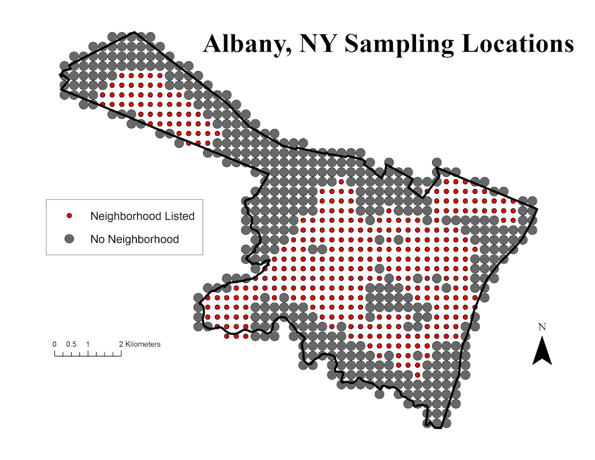
See my python code at the end of the post to see how I extracted this info. given an input lat-lng. In the reverse geo api they return multiple addresses – but I only examine the first returned address and look for a neighborhood. (So I could have missed some neighborhoods this way – it would take more investigation.)

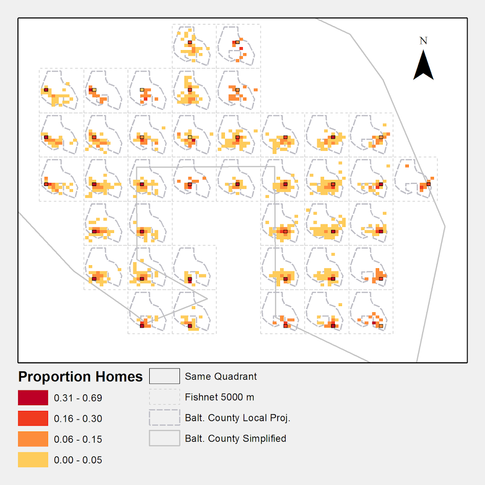
Given the input fishnet I then dissolved the neighborhood labels into areas. Google has quite a few more specific neighborhoods than me.

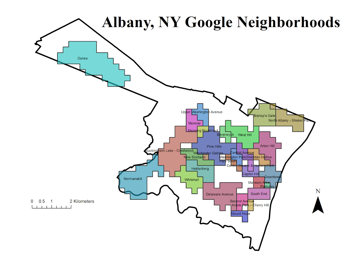
I’ve never really made much of a distinction between West Hill and Arbor Hill – although the split is clearly at Henry Johnson. Also I tend to view Pine Hill as the triangle between Western and Central before the State campus – but Google and others seem to disagree with me. What I call the Pinebush Google calls the Dunes. Dunes is appropriate, because it actually has sand dunes, but I can’t recall anyone referring to it as that. Trees are pretty hard to come by in Arbor Hill though, so don’t be misled. Also kill is Dutch for creek, so you don’t have to worry that Normanskill is such a bad place (even if your name is Norman).

For a third opinion, see albany.com

You can see more clearly in this map how Pine Hill’s area goes south of Madison. Google maps has a fun feature showing related maps, and so they show a related map on someones take for where law students should or should not get an apartment. In that map you can see that south of Madison is affectionately referred to as the student ghetto. That comports with my opinion as well, although I did not think putting student ghetto was appropriate for my basemap for a journal article!

People can’t seem to help but shade Arbor Hill in red. Which sometimes may be innocent – if red is the first color used in defaults (as Arbor Hill will be the first neighborhood in an alphabetic list). But presumably the law student making the apartment suggestions map should know better.

In short, it would be convenient for me (as a researcher) if everyone could agree with what a neighborhood is and where its borders are, but that is not reality.


Here is the function in Python to grab the neighborhood via the google reverse geocoding API. Here if it returns anything it grabs the first address returned and searches for the neighborhood in the json. If it does not find a neighborhood it returns None.

#Reverse geocoding and looking up neighborhoods
import urllib, json

def GoogRevGeo(lat,lng,api=""):
  base = r"https://maps.googleapis.com/maps/api/geocode/json?"
  GeoUrl = base + "latlng=" + str(lat) + "," + str(lng) + "&key=" + api
  response = urllib.urlopen(GeoUrl)
  jsonRaw = response.read()
  jsonData = json.loads(jsonRaw)
  neigh = None
  if jsonData['status'] == 'OK':
    for i in jsonData['results'][0]['address_components']:
      if i['types'][0] == 'neighborhood':
        neigh = i['long_name']
        break
  return neigh

Some GIS data scraping adventures: Banksy graffiti and gang locations in NYC

I’ve recently scraped some geographic data that I may use in my graduate level GIS course. I figured I would share with everyone, and take some time to describe for others how I scraped the data.

So to start, if you read an online article and it has a webmap with some GIS data in it – the data exists somewhere. It won’t always be the case that you can actually download the data, but for the most current and popular interactive mapping tools, the data is often available if you know where to look.

For example, I asked on the GIS stackexchange site awhile ago how can you download the point data in this NYC homicide map from the Times. I had emailed the reporters multiple times and they did not respond. A simple solution the answerers suggested was to use website developer tools to see what was being loaded when I refreshed the page. It happened that the map is being populated by a two simple text files (1,2).

It may be an interesting project to see how this compares (compiling via news stories) versus official data, which NYC recently released going back to 2006. Especially since such crowdsourced news datasets are used for other things, like counting mass shootings.

The two example mapping datasets I provide below though are a bit different process to get the underlying data – but just as easy. Many current webmaps use geojson files as the backend. What I did for the two examples below is I just looked at the html source for the website, and look for json data formats – links that specify “js” or “json” extensions. If you click through those external json links you can see if they have the data.

The other popular map type though comes from ESRI. You can typically find an ESRI server populating the map, and if the website has say a parcel data lookup you can often find an ESRI geocoding server (see here for one example of using an ESRI geocoding api). The maps though unfortunately do not always have exposed data. Sometimes what looks like vector data are actually just static PNG tiles. Council Districts in this Dallas map are an example. If you dig deep enough, you can find the PNG tiles for the council districts, but that does not do anyone much good. Pretty much all of those layers are available for download from other sources though. A similar thing happens with websites with crime reports, such as RAIDS Online or CrimeReports.com. They intentionally build the web map so you cannot scrape the data.

So that said, before we go further though – it should go without saying that you should not steal/plagiarize people’s articles or simply rip-off their graphics. Conducting new analysis with the publicly available data though seems fair game to me.

Banksy Taggings in NYC

There was a recent stink in the press about Kim Rossmo and company using geographic offender profiling to identify the likely home location of the popular graffiti artist Banksy. Here is the current citation of the journal article for those interested:

Hauge, M. V., Stevenson, M. D., Rossmo, D. K., and Le Comber, S. C. (2016). Tagging banksy: using geographic profiling to investigate a modern art mystery. Journal of Spatial Science, pages 1-6. doi:10.1080/14498596.2016.1138246

The article uses data from Britain, so I looked up to see if his taggings in other places was available. I came across this article showing a map of locations in New York City. So I searched where the data was coming from, and found the json file that contains the point data here. I just built a quick excel spreadsheet to parse the data, and you can download that spreadsheet here.

Gang Locations

This article posts a set of gang territories in NYC. This is pretty unique – I am unfamiliar with any other public data source that identifies gang territories. So I figured it would be a potential fun project for students in my GIS course – for instance in overlaying with the 311 graffiti data.

Again the data at the backend is in json format, and can be found here. To convert this data to a shapefile is a bit challenging, as it has points, lines and polygons all in the same file. What I did was buffer the lines and points by a small amount to be able to stuff them all in one shapefile. A zip file of that shapefile can be downloaded here.

Drop me a note if you use this data, I’d be interested in your analyses! Hence why I am sharing the data for others to play with 🙂

Adding a command button to a toolbar in ArcGIS

I’m currently teaching a graduate level class in Crime Mapping using ArcGIS. I make my own tutorials from week to week, and basically sneak in generic pro-tips for using the software while students are doing other regular types of analyses. I can only subject my students to so much though – but here is one I have found useful, adding a regularly used button to a toolbar.

I use CrimeStat to generate kernel densities from point data, so as of V10 whenever I want to make a classified raster map I get this error:

V9 it used to just do this for you automatically :(.

I typically make classified raster maps simply because I think they look nicer than continous ones. My continuous ones always look fuzzy, whereas having discrete cuts you can focus attention on particular hot spot areas. It is arbitrary for sure – but that is something we need to learn to live with when making maps.

So in class I had students open ArcToolBox, navigate down the tree, and find the Calculate Statistics tool for rasters. In my personal set up though I do this enough that I added the button to my toolbar. So first, go to the file menu and in customize -> toolbars make sure you have the spatial analyst toolbar selected. (Here is a kernel density grd file to follow along with if you want.)

Now in the right hand most edge of the new spatial analyst toolbar, left click on the little downward pointing arrow and select Customize. (Sorry, my toolbar is a bit crowded!)

In the customize window that pops up, select the Commands tab. Now in this window you can select any particular command and then drag it onto any toolbar. Here I go to Data Management in the left hand categories area, and then scroll down till I find the Calculate Statistics button.

Then I left click on the Calculate Statistics row, hold down the mousebutton, and drag it to my toolbar.

Now you are done, and ArcGIS saves this button on the toolbar when making future maps. You can change the icon if you want, but there are tooltips when hovering over the icon (so even if you have multiple hammers on your toolbars it only takes a second to browse between them).

Using Python to grab Google Street View imagery

Update: I have been asked several times over the years for help on this. In response I have made a simple GUI tool, given a list of addresses and a download folder location, will download all of the images. Applications are websites listing properties and marketers for mailings.

The tool costs $300, Check out the CRIME De-Coder Store to purchase.


I am at it again with using Google data. For a few projects I was interested in downloading street view imagery data. It has been used in criminal justice applications as a free source for second hand systematic social observation by having people code aspects of disorder from the imagery (instead of going in person) (Quinn et al., 2014), as estimates of the ambient walking around population (Yin et al., 2015), and examining criminogenic aspects of the built environment (Vandeviver, 2014).

I think it is just a cool source of data though to be honest. See for example Phil Cohen’s Family Inequality post in which he shows examples of auctioned houses in Detroit over time.

Using the Google Street View image API you can submit either a set of coordinates or an address and have the latest street view image returned locally. This ends up being abit simpler than my prior examples (such as the street distance API or the places API) because it just returns the image blob, no need to parse JSON.

Below is a simple example in python, using a set of addresses in Detroit that are part of a land bank. This function takes an address and a location to download the file, then saves the resulting jpeg to your folder of choice. I defaulted for the image to be 1200×800 pixels.

import urllib, os

myloc = r"C:\Users\andrew.wheeler\Dropbox\Public\ExampleStreetView" #replace with your own location
key = "&key=" + "" #got banned after ~100 requests with no key

def GetStreet(Add,SaveLoc):
  base = "https://maps.googleapis.com/maps/api/streetview?size=1200x800&location="
  MyUrl = base + urllib.quote_plus(Add) + key #added url encoding
  fi = Add + ".jpg"
  urllib.urlretrieve(MyUrl, os.path.join(SaveLoc,fi))

Tests = ["457 West Robinwood Street, Detroit, Michigan 48203",
         "1520 West Philadelphia, Detroit, Michigan 48206",
         "2292 Grand, Detroit, Michigan 48238",
         "15414 Wabash Street, Detroit, Michigan 48238",
         "15867 Log Cabin, Detroit, Michigan 48238",
         "3317 Cody Street, Detroit, Michigan 48212",
         "14214 Arlington Street, Detroit, Michigan 48212"]

for i in Tests:
  GetStreet(Add=i,SaveLoc=myloc)

Dropbox has a nice mosaic view for a folder of pictures, you can view all seven photos here. Here is the 457 West Robinwood Street picture:

In my tests my IP got banned after around 100 images, but you can get a verified google account which allows 25,000 image downloads per day. Unfortunately the automatic API only returns the most recent image – there is no way to return older imagery nor know the date-stamp of the current image. (You technically could download the historical data if you know the pano id for the image. I don’t see any way though to know the available pano id’s though.) Update — as of 2018 there is now a Date associated with the image, specifically a Year-Month, but no more specific than that. Not being able to figure out historical pano id’s is still a problem as far as I can tell as well.

But this is definitely easier for social scientists wishing to code images as opposed to going into the online maps. Hopefully the API gets extended to have dates and a second API to return info. on what image dates are available. I’m not sure if Mike Bader’s software app is actually in the works, but for computer scientists there is a potential overlap with social scientists to do feature extraction of various social characteristics, in addition to manual coding of the images.


Update: here is a version that works for python 3+. Currently you need to have a key, no more getting a few free images before being cut off.

# For Python Versions 3+
# Tested V3.10 on 12/15/2021
import os
import urllib.parse
import urllib.request

myloc = r"??????????????" #replace with your own location
key = "&key=" + "????????????" #you need an actual key now!!

def GetStreet(Add,SaveLoc):
  base = "https://maps.googleapis.com/maps/api/streetview?size=1200x800&location="
  MyUrl = base + urllib.parse.quote_plus(Add) + key #added url encoding
  fi = Add + ".jpg"
  urllib.request.urlretrieve(MyUrl, os.path.join(SaveLoc,fi))

Tests = ["457 West Robinwood Street, Detroit, Michigan 48203",
         "1520 West Philadelphia, Detroit, Michigan 48206",
         "2292 Grand, Detroit, Michigan 48238",
         "15414 Wabash Street, Detroit, Michigan 48238",
         "15867 Log Cabin, Detroit, Michigan 48238",
         "3317 Cody Street, Detroit, Michigan 48212",
         "14214 Arlington Street, Detroit, Michigan 48212"]

for i in Tests:
  GetStreet(Add=i,SaveLoc=myloc)

The spatial consistency of bar locations – Buffalo 1901 vs. 2015

Part of my work I’m interested in the correlates of crime at very small places, particularly aspects of the built environment. Part of the difficulty of this work though is that some aspects of the built environment change very slowly. I often just anecdotally give bars as an example – when a bar goes under it often just gets replaced by another bar. So for example if I want to make an estimate of how much crime would decrease if you took a bar away, it is difficult looking at historical data because most of the time when a bar goes away it is just replaced by another in a short time span.

But admittedly this perception was just based on my anecdotal experiences. So when I saw some historical maps John Krygier posted of saloons I wanted to put a pretty strict test to my assertion. Here is a map of saloons in Buffalo (circa 1901 on John’s website):

I grabbed the current locations of places licensed to sell alcohol in New York State via the open data portal and geocoded those in Buffalo. (This includes things like grocery stores as well as bars.) I did a mediocre job trying to digitize the old map (here is the digitized image), and here we can see the overlap between the current and the historical locations. Zoom into the area with the blue icons to see the historical locations.

So we can see that my baseline of bars not changing is not accurate for this for this extreme comparison. If you zoom out you can see that there is a higher concentration of bars just to the west, so I wonder if over time there was a shift of these bar locations.

John has some more examples of historical saloon maps in Baltimore plus San Francisco and New York City (in the same post with Buffalo). I’d be interested to see those locations as well if someone takes the time to replicate this.

I may have to think more seriously about evaluating the effect of bars over time, and seeing if things like bars losing their licenses because of violations result in crime decreases.

Cartography and GIS special issue on Crime Mapping

My paper, Visualization techniques for journey to crime flow data, has been recently published in a special issue in CaGIS on crime mapping. Always feel free to email me for off-prints of published papers, but the pre-print of this one I posted on SSRN as well.

There is an annoying error that crept into the paper, in that the footnote linking to the results to replicate the maps and graphs says “REDACTED FOR ANONYMITY” – which is my fault for not pointing it out to the copy-editor. The files are available here. They are certainly not easy to walk through, so if you want help replicating any of the maps for your own data and can’t figure out my code feel free to send me an email. I would like to make an R package to make maps like below eventually, but that is just not going to happen in the forseeable future.

Some more on Network distances vs Geographic distances intra-city

A prior post on analyzing distances looked at geographic versus network (road) distances between zip codes in New York and one particular location. Over the large distances the correlation ended up being 0.99. But most crime analysis applications will be within one city, so restricting the distances there will the correlation be just as high? I conducted some analysis in Albany, NY to see if this was the case.

First I took a set of 2,640 street segments and intersections in Albany, defined as basically having over 1 reported crime between 2000 through 2013. (This is a pretty good proxy for places where people are actually located in the city, so places where people might actually travel from/to.) Here is a map of those points showing the coverage.

I then made the 2,640^2 pairs, and then took a random sample of 2,300 of those pairs to calculate the geographic versus the network distance (calculating the network distance using the google distance API). Here is a flow map, again showing it has pretty good coverage of the city.

In this sample the correlation between the network distance and the geographic distance is 0.94, and below is the scatterplot. The red line is the line of equality, so we can see the network distance is always larger.

Making the graph on log scales basically takes away the heteroscedasticity, and shows some short distance outliers.

I then fit a regression of equation of log(Network Distance) ~ Intercept + b_0*log(Geo Distance), and then calculate the studentized residuals. Here is a small multiple flow map of those locations categorized by the truncated studentized residuals. I plotted flows under 200 meters as a red dot, as otherwise they basically have no area on the map to visualize. There are a few notable patterns, the -1 residuals (so closer network and geo distances) are locations along what looks like Central, Washington, Western and New Scotland (running east-west) and Broadway/Pearl (running north-south). So basically straight, major thoroughfares.

It is probable that if more locations in the isthmus and the south western part of the city were selected the distances would be not so nice, but the isthmus itself is largely the Pine Bush park, and the south western part is on the periphery of residential neighborhoods. Exporting the high residuals, what happens in the google distance API is that they are short trips on one way streets, and the to and from and going against the one way. I will have to investigate if you can set the google API to use walking distances to ignore this (as this wasn’t intended as a directed flow like that). Or just learn how to use the CrimeStat or network analysis in ArcMap distance calculation tools!

So although using network distances consistently increases the distances between points, they are still highly correlated, even for shorter in city patterns. If I fixed the flows going against one way streets it would likely be an even higher correlation.

Using the New York State Online Geocoding API with Python

I’ve been very lucky doing geographic analysis in New York state, as the majority of base map layers I need, and in particular streets centerline files for geocoding, are available statewide at the NYS GIS Clearing house. I’ve written in the past how to use various Google API’s for geo data, and here I will show how one can use the NYS SAM Address database and their ESRI online geocoding service. I explored this because Google’s terms of service are restrictive, and the NYS composite locator should be more comprehensive/up to date in matches (in theory).

So first, this is basically the same as with most online API’s (at least in my limited experience), submit a particular url and get JSON in return. You just then need to parse the JSON for whatever info you need. This is meant to be used within SPSS, but the function works with just a single field address string and returns the single top hit in a list of length 3, with the unicode string address, and then the x and y coordinates. (The function is of course a valid python function, so you could use this in any environment you want.) The coordinates are specified using ESRI’s WKID (see the list for projected and geographic coordinate systems). In the code I have it fixed as WKID 4326, which is WGS 1984, and so returns the longitude and latitude for the address. When the search returns no hits, it just returns a list of [None,None,None].

*Function to use NYS geocoding API.
BEGIN PROGRAM Python.
import urllib, json

def ParsNYGeo(jBlob):
  if not jBlob['candidates']:
    data = [None,None,None]
  else:
    add = jBlob['candidates'][0]['address']
    y = jBlob['candidates'][0]['location']['y']
    x = jBlob['candidates'][0]['location']['x']
    data = [add,x,y]
  return data

def NYSGeo(Add, WKID=4326):
  base = "http://gisservices.dhses.ny.gov/arcgis/rest/services/Locators/SAM_composite/GeocodeServer/findAddressCandidates?SingleLine="
  wkid = "&maxLocations=1&outSR=4326"
  end = "&f=pjson"
  mid = Add.replace(' ','+')
  MyUrl = base + mid + wkid + end
  soup = urllib.urlopen(MyUrl)
  jsonRaw = soup.read()
  jsonData = json.loads(jsonRaw)
  MyDat = ParsNYGeo(jsonData)
  return MyDat

t1 = "100 Washington Ave, Albany, NY"
t2 = "100 Washington Ave, Poop"

Out = NYSGeo(t1)
print Out

Empt = NYSGeo(t2)
print Empt
END PROGRAM.

So you can see in the code sample that you need both the street address and the city in one field. And here is a quick example with some data in SPSS. Just the zip code doesn’t return any results. There is some funny results here though in this test run, and yes that Washington Ave. extension has caused me geocoding headaches in the past.

*Example using with SPSS data.
DATA LIST FREE / MyAdd (A100).
BEGIN DATA
"100 Washington Ave, Albany"
"100 Washinton Ave, Albany"
"100 Washington Ave, Albany, NY 12203"
"100 Washington Ave, Albany, NY, 12203"
"100 Washington Ave, Albany, NY 12206"
"100 Washington Ave, Poop"
"12222"
END DATA.
DATASET NAME NY_Add.

SPSSINC TRANS RESULT=GeoAdd lon lat TYPE=100 0 0 
  /FORMULA NYSGeo(Add=MyAdd).

LIST ALL.

Using Google Fusion Tables to make some maps!

In the past to share interactive maps with others I’ve used BatchGeo and CartoDB. BatchGeo is super easy to geocode a few incidents, and CartoDB has a few more stylistic options (including some very cool animations). Both of these projects have a limit on the number of points you can map with the free service though. The new Google maps allows you make similar products to BatchGeo and CartoDB, in that you can upload a csv file or kml and then do some light editing of the points, and then embed an iframe in a website if you want (I wish Google Maps had a time slider like Google Earth does). Here is an example from my PhD of a few locations that one of my original models did a very poor job of predicting the amount of crime at the street midpoint or intersection.

But a few recent projects I wanted to place many more geographies on the map than these free versions allow. ArcGIS online is pretty slick in my few tests, but I am settling on Google Fusion tables for the ability to link the geographies and data tables (plus the ability to filter is very nice). Basically you can upload your data table and kml in seperate Fusion tables and then merge them to create your own polygons with associated data. Here is another example from my dissertation and embedded map below.

Basically what I do is make a set of units of analysis based on street mid-points and intersections. I then divide the city up based on the Thiessen polygons of those sets of points for the allocation of different areal measures. E.g. I can calculate the overlap of the Thiessen polygon with the area of sidewalks.

I’m using Google Fusion tables for some other projects in which I want people within the PD to be able to interactively explore the data. My main interest in these slippy maps are that you can pan and zoom – and with a static map it is hard to recreate all of the potential views a consumer of the map wants. I can typically make a nicer overview map of the forest or any general data patterns in a static map, but if I think the user of the map will want to zoom in to particular locations these interactive maps meet that challenge. Pop-ups allow for a brief digging into the data as well, but don’t allow for visualizing patterns. Fusion tables are very limited though it the styling of the geography. (All of these free versions are pretty limited, but the Fusion tables are especially restrictive for point symbology and creating choropleth classes).

Using these maps has a trade off when sharing with the PD though. They are what I would call semi-public, in that if you want others to be able to view the map you can share a link, but anyone with the link can see the map. This prevents sharing of intimate information on the map that might be possibly leaked. (For the ability to have access control to more sensitive information, e.g. a user has to sign on to a secure website, I know Bair analytics offers paid for products like that – probably some of the prior web map apps I mentioned do so as well.) I’ve made them in the past for Troy P.D., but I really have no idea how often they were used – so other analysts let me know in the comments if you’ve had success with maps like these disseminating info. within the police department.

I’m getting devilishly close to finishing my dissertation, and I will post an update and link when the draft is complete. My prospectus can be seen here, and the linked maps are part of some supplemental material I compiled. The supplemental info. should provide a little more details on what the maps are showing.

What is up with 3d graphics for book covers?

The other day in Google books I noticed Graphics for Statistics and Data Analysis with R by Kevin Keen in the related book section. What caught my eye was not the title (there have to be 100+ related R books at this point) but the really awful 3d pie chart.

Looking at the preview on google books this appears to be an unfortunate substitution. The actual cover has a much more reasonable set of surface plots and other online book stores (e.g. Amazon) appear to have the correct cover.

I suspect someone at CRC Press used some stock imagery for the cover, and unfortunately the weird 3d pie graph has been propagated to the google book preview without correction.

This reminded me of a few other book covers in cartography and data visualization though that I find less than appealing. Now, I’m not saying here to judge a book by its cover, and I have not read all of the books I will point to here. But I find the use of 3d graphics in book covers in the data visualization field to be strange and bordering cognitive dissonance with the advice most of the authors give.

First I’ll start with a book I have read, and would suggest to everyone, Thematic cartography and geographic visualization by Slocum et al. I have the 2005 version, and it is dawned by this 3d landscape. (Sorry this is the largest image I can find online – other editions I believe have different covers.)

The multivariate display of data is admirable – so for exploratory analysis you could make a reasonable argument for the use of proportional sized circles superimposed on the choropleth map. The use of 3d in this circumstance though is gratuitous, and the extreme perspective hides much of the data while highlighting the green hills in the background.

The second mapping book I have slight reservations about critiquing the cover (I am on the job market!). I have not read the book, so I can not say anything about its contents. But roaming the book displays at an ASC conference I remember seeing this cover, GIS and Spatial Analysis for the Social Sciences: Coding, Mapping, and Modeling by Nash and Asencio.

This probably should not count in the other 3d graphics I am showing. The bar columns do have shading for 3d perspective – but the map otherwise is 2d. But the spectral color scheme is an awful choice. The red in the map tends to stand out the most – which places with zero crimes I don’t think you want to make that impression. The choropleth colors appear to be displaying the same data as the point data. The point data are so clustered that the choropleth can only be described as misleading – which may be a good point in text for side by side maps – but on the cover? Bar locations seem to be unrelated (as we might expect for juvenile crime) but they are again aggregated to the (probably) census units – making me question if the aggregation obfuscates the relationship. Bars are not available from the census – so it is likely this aggregation was intentional. I have no idea about the content of the book and I will likely get it and do an overall review of all crime mapping books sometime. But the cover is unambiguously a bad map.

The last book cover with 3d graphics (related to data-visualization) that I immediately remembered was R For Dummies by Meys and de Vries.

Now this when you look close really is not bad. It is not a graph on the cover, but a set of winding, hexagon cylinder stairsteps. So the analogy of taking small steps is fine – but the visual similarity to other statistical 3d graphics is clear. Consider the SPSS For Dummies book by Griffith.

Now that is an intentional, 3d chart made up of tiny blocks, with a trend line if you look closely, shadowed by cigarette like red bars in the background. At least this is so strange (and not possible in statistical software) that this example would never be confused with an actual reasonable statistical graphic. The Dummies series has such brand recognition as well that the dominant part of the cover might be the iconic yellow and type, as opposed to the inset graphic.

Not wanting to leave other software out of the loop, I looked for examples for SAS and Stata. SAS has a reasonable 3d cover in SAS System for Statistical Graphics by Friendly.

Short sidetrack story: I first learned statistical programming using SAS back in undergrad days at Bloomsburg University. Default graphics for SAS at that point (04-08) I believe were still the ASCII art looking things (at least that is what I remember). During our last meeting for my last statistics class – one of the other students showed me you could turn on the ODS output to html – and tables and graphs were by default pretty nice. I since have not had a need to use SAS.

This 3d cover by Friendly is arguably a reasonable use of 3d. 3d graphs are hard to navigate, and the use the anchors connecting the observations to the non-linear surface more easily associate a point with below or above the surface. It is certainly difficult though to understand the fit of the function – so likely a series of bivariate graphs would be more intuitive – especially given the meager number of points. I suspect the 3d on the cover is for the same reason 3d graphics were used in the other covers – because it looks cooler to book marketers!

Stata managed to debunk the 3d graph trends – I could not find any example Stata books with 3d graphics. Nick Cox’s newer collection of his Speaking Stata series though has some interesting embellishments.

While in isolation all of the graphs are fine – I’m sure Cox would not endorse the gratuitous use of color gradients in the graphics (I don’t think svg like gradients like that are even possible in Stata graphics). The ternary diagrams show nothing but triangles as well – so I don’t think such gradients are a good idea in any case for simply the background of the plot. Such embellishments could actually decode data, but in the case of bar graphs do not likely hurt or help with understanding the plot. When such gradients are used as the background though they likely compete with the actual data in the plot. Stata apparently can do 3d graphs – so I might suggest I write a book on crime modelling (published by Stata press) and insert a 3d graph on the cover (as this is clearly a niche in the market not currently filled!) I might have to make room for Chernoff faces somewhere on the front or back cover as well.

So maybe I am just seeing things in the examples of 3d covers. If anyone has any insight into how these publishers choose the covers let me know – or if you have other examples of bad book cover examples of data vizualization! Since most of my maps and graphs are pretty dull in 2d I might just outsource the graphic design if I made a book.