So one of the problems I have been thinking about at work is assessing spatial access to providers. Some common metrics are ‘distance to nearest’, or combining distance as well as total provider capacity into one metric, the two-step floating catchment method (2SFCA).

So imagine we are trying to evaluate the coverage of opioid treatment facilities relative to the spatial distribution of people abusing opioids. Say for example we have two areas, A and B. Area A has a facility that can treat 50 people, but has a total of 100 people who need service. Now Area B has no treatment provider, but only has 10 people that need service.

If you looked at distance to nearest provider, location B would look worse than A. So you may think to yourself – we should open up a facility in Area B. But if you look at the total number of people, as well as the capacity of the treatment provider in Area A, it would probably be a better investment to expand the capacity of treatment center A. It has more potential demand.

The 2SFCA partially captures this, but I am going to show a linear programming approach that can decompose the added benefit of adding capacity to a particular provider, or adding in potential new providers. I have the posted these functions on github, but can walk through the linear programming model, and how to assess potential policy interventions in that framework.

So first lets make just a simple set of data, we have 10 people with XY coordinates, and 2 service providers. The two service providers have capacity 3 and 5, so we cannot cover 2 of the people.

# Python example code
import numpy as np
import pandas as pd
import pulp

# locations of people
id = range(10)
px = [1,1,3,3,4,5,6,6,9,9]
py = [2,8,1,8,4,6,1,2,5,8]
peop = pd.DataFrame(zip(id,px,py),columns=['id','px','py'])

# locations of 2 providers & capacity 3/5
hid = [1,2]
hx = [1,8]
hy = [1,8]
hc = [3,5] # so cant cover 2 people
prov = pd.DataFrame(zip(hid,hx,hy,hc),columns=['hid','hx','hy','hc'])

Now for the subsequent model I show, it is going to assign the people to the nearest possible provider, given the distance constraints. To make the model feasible, we need to add in a slack provider that can soak up the remaining people not covered. We set this location to somewhere very far away, so the model will only assign people to this slack provider in the case no other options are available.

# add in a slack location to the providers
# very out of the way and large capacity
prov_slack = prov.iloc[[0],:].copy()
prov_slack['hid'] = 999
prov_slack['hx'] = 999
prov_slack['hy'] = 999
prov_slack['hc'] = peop.shape[0]
prov_add = pd.concat([prov,prov_slack],axis=0)

Now the decision model looks at all pairwise combinations between people and providers (potentially eliminating combinations that are too far away to be reasonable). So I do the cross join between the people/providers, and then calculate the Euclidean distance between them. I set the distance for the slack provider to a very high value (here 9999).

# distance between people/providers
peop['const'] = 1
prov_add['const'] = 1
cross = pd.merge(peop,prov_add,on='const')
cross['dist'] = np.sqrt( (cross['px']-cross['hx'])**2 + 
                         (cross['py']-cross['hy'])**2 )
cross.set_index(['id','hid'],inplace=True)
# setting max distance for outside provider to 9999
cross.loc[cross.xs(999,level="hid",drop_level=False).index,"dist"] = 9999

Now we are ready to fit our linear programming model. First our objective is to minimize distances. (If all inputs are integers, you can use continuous decision variables and it will still return integer solutions.)

# now setting up linear program
# each person assigned to a location
# locations have capacity
# minimize distance traveled

# Minimize distances
P = pulp.LpProblem("MinDist",pulp.LpMinimize)

# each pair gets a decision variable
D = pulp.LpVariable.dicts("DA",cross.index.tolist(),
                          lowBound=0, upBound=1, cat=pulp.LpContinuous)

# Objective function based on distance
P += pulp.lpSum(D[i]*cross.loc[i,'dist'] for i in cross.index)

And we have two types of constraints, one is that each person is assigned a single provider in the end:

# Each person assigned to a single provider
for p in peop['id']:
    provl = cross.xs(p,0,drop_level=False).index
    P += pulp.lpSum(D[i] for i in provl) == 1, f"pers_{p}"

As a note later on, I will expand this model to include multiple people from a single source (e.g. count of people in a zipcode). For that expanded model, this constraint turns into pulp.lpSum(...) == tot where tot is the total people in a single area.

The second constraint is that providers have a capacity limit.

# Each provider capacity constraint
for h in prov_add['hid']:
    peopl = cross.xs(h,level=1,drop_level=False)
    pid = peopl.index
    cap = peopl['hc'].iloc[0] # should be a constant
    P += pulp.lpSum(D[i] for i in pid) <= cap, f"prov_{h}"

Now we can solve the model, and look at who was assigned to where:

# Solve the model
P.solve(pulp.PULP_CBC_CMD()) 
# CPLEX or CBC only ones I know of that return shadow
pulp.value(P.objective) #print objective 20024.33502494309


# Get the person distances
res_pick = []
for ph in cross.index:
    res_pick.append(D[ph].varValue)

cross['picked'] = res_pick
cross[cross['picked'] > 0.99]

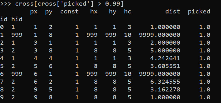
So we can see two people were assigned the slack provider 999. Note that some people are not even assigned the closest – person 7 (6,2) is assigned to provider 2 at a distance of 6.3, it is only a distance of 5.1 away from provider 1. Because provider 1 has limited capacity though, they are assigned to provider 2 in the end.

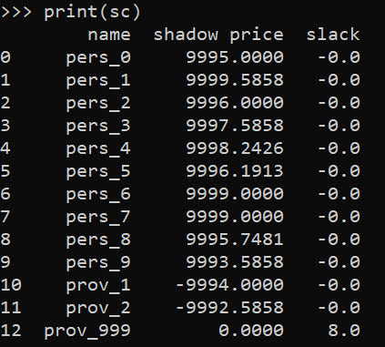
In this framework, we can get the shadow price for the constraints, which says if we relax the constraint, how much it will improve our objective value.So if we add 1 capacity to provider 1, we will improve our objective by -9994.

# Get the shadow constraints per provider
o = [{'name':name, 'shadow price':c.pi, 'slack': c.slack} 
     for name, c in P.constraints.items()]
sc = pd.DataFrame(o)
print(sc)

I have helper functions at the github link above, so I don’t need to go through all of these motions again. You input your people matrix and the field names for the id, x, y, totn values.

And then you input your provider matrix with the field names for the providerid, x, y, prov_capacity (note this is not the matrix with the additional slack provider, my code adds that in automatically). The final two arguments limit the potential locations (e.g. here saying can’t assign a person to a provider over 12 distance away). And the last argument sets the super high distance penalty to people are not assigned.

# load in model functions
from assign_funcs import ProvAssign

# Const=1 is the total people per area
m1 = ProvAssign(peop,
                ['id','px','py','const'],
                prov,
                ['hid','hx','hy','hc'],
                12,
                9999)

m1.solve(pulp.PULP_CBC_CMD())
# see the same objective as before

Now we can go ahead and up our capacity at provider 1 by 1, and see how the objective is reduced by -9994:

# if we up the provider capacity for
# prov by 1, the model objective goes 
# down by -9994
prov['hc'] = [4,5]

m2 = ProvAssign(peop,
                ['id','px','py','const'],
                prov,
                ['hid','hx','hy','hc'],
                12,
                9999)
m2.solve(pulp.PULP_CBC_CMD())
m1.obj - m2.obj # 9994!

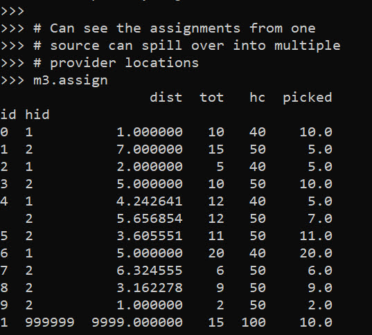
Like I said, I extended this to the scenario that you don’t have individual people, but have multiple counts of people in a spatial area. What can happen in this scenario is one source location can send people to multiple providers. Here you can see that source location 4 (total of 12 people), 5 were sent to provider 1, and 7 were sent to provider 2.

# Can make these multiple people, 100 total
peop['tot'] = [10,15,5,10,12,11,20,6,9,2]
prov['cap'] = [40,50] # should assign 10 people to slack

m3 = ProvAssign(peop,
                ['id','px','py','tot'],
                prov,
                ['hid','hx','hy','cap'],
                12,
                9999)
m3.solve(pulp.PULP_CBC_CMD())
# Can see the assignments from one
# source can spill over into multiple
# provider locations
m3.assign

So one of the things I like about this approach I already showed, we can do hypothetical scenarios ‘add capacity’ and see how it improves overall travel. Another potential intervention is to just place dummy 0 capacity providers over the study area, then look at the shadow constraints to see the best locations to open new facilities. Here I add in a potential provider at location (5,5).

# Can add in hypothetical providers with
# no capacity (make new providers)
# and check out the shadow
p2 = prov_slack.copy()
p2['hid'] = 10
p2['hx'] = 5
p2['hy'] = 5
p2['hc'] = 0
p2['cap'] = 0
prov_add = pd.concat([prov,p2],axis=0)


m4 = ProvAssign(peop,
                ['id','px','py','tot'],
                prov_add,
                ['hid','hx','hy','cap'],
                10,
                9999)

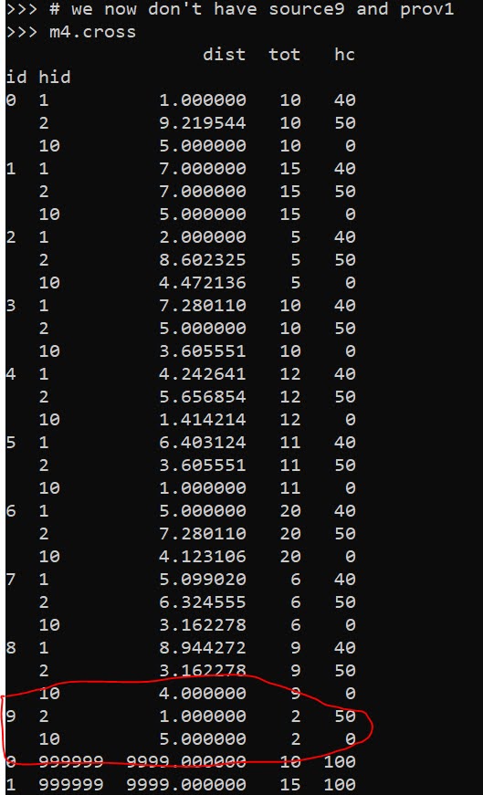
# we now don't have source9 and prov1
m4.cross

Here in the code, I also have a function to limit potential assignments. Here if I set that limit to 10, it only just prevents id 9 (9,8) from being assigned to provider 1 (1,1), which is a distance of 10.6 away. This is useful with larger datasets, in which you may not be able to fit all of the pairwise distances into memory and model. (Although this model is pretty simple, you may be able to look at +1 million pairwise combos and solve in a reasonable time with open source solvers.)

Now we can go ahead and solve this model. I have a bunch of helper functions as well, so after solving we can check out the shadow price matrix:

# Solve m4 model
m4.solve(pulp.PULP_CBC_CMD())

# can see the new provider 10
# if we added capacity would
# decrease distance travelled by -9996.2426
m4.shadow

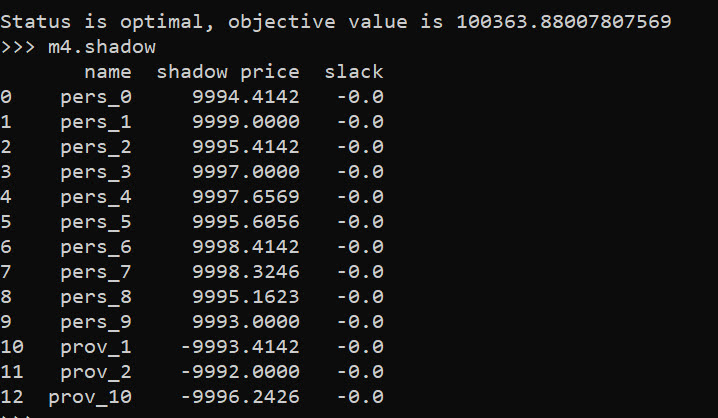
And based on this, it does look like we will have the best improvement by adding capacity at our hypothetical new provider 10, as oppossed to adding capacity at provider 1 or 2. Lets see what happens if you add 10 capacity to our hypothetical provider:

# Now lets add capacity for new provider
# by 10, should the objective go down
# by 10*-9996.2426 ?
prov_add['cap'] = [40,50,10]

m5 = ProvAssign(peop,
                ['id','px','py','tot'],
                prov_add,
                ['hid','hx','hy','cap'],
                12,
                9999)
m5.solve(pulp.PULP_CBC_CMD())

# Not quite -9996.2 but close!
(m5.obj - m4.obj)/10

We can see that the objective was not quite reduced by the expected, but is close. If it is not feasible to add a totally new provider, but simpler to give resources to expand current ones, we can see what will happen if we expand provider 1 by 10.

# we could add capacity
# to provider 1 by 10
# as well
prov_add['cap'] = [50,50,0]

m6 = ProvAssign(peop,
                ['id','px','py','tot'],
                prov_add,
                ['hid','hx','hy','cap'],
                10,
                9999)
m6.solve(pulp.PULP_CBC_CMD())

# Not quite -9993.4 but close!
(m6.obj - m4.obj)/10

In addition to doing different policy interventions in this approach, I provide different metrics to assess distance traveled and coverage. So going back to model 4, we can look at which areas have limited coverage. It only ends up that source area 1 has 10/15 people not covered. The rest of the areas are covered.

# Can look at sources and see stats
# for distance travelled as well
# as potential non-coverage
m4.source_stats

The fields are Trav is the average distance travelled for people who are covered (so could have high coverage but those people have to go a ways). Tot is the total number of people within that particular source area, and picked/not-covered are those assigned a provider/not assigned a provider (so go to the slack) respectively.

I additionally I have stats available rolled up to providers, mostly based on the not covered nearby. One way that the shadow doesn’t work, if you only have 10 people nearby, it doesn’t make sense to expand capacity to any more than 10 people. Here you can see the shadow price, as well as those not covered that are nearby to that provider.

# Can look at providers
# and see which ones would result in
# most reduced travel given increased coverage
# Want high NotCover and low shadow price
m4.prov_stats

The other fields, hc is the listed capacity. Trav is the total travel for those not covered. The last field bisqw, is a way to only partially count not covered based on distance. It uses the bi-square kernel weight, based on the max distance field you provided in the model object. So if many people are nearby it will get a higher weight.

Here good add capacity locations are those with low shadow prices, and high notcovered/bisqw fields.

Note these won’t per se give the best potential places to add capacity. It may be the best new solution is to spread out new capacity – so here instead of adding 10 to a single provider, add a few to different providers.

You could technically figure that out by slicing out those leftover people in the m4.source_stats that have some not covered, adding in extra capacity to each provider, and then rerunning the algorithm and seeing where they end up.

Again I like this approach as it lets you articulate different policy proposals and see how that changes the coverage/distance travelled. Although no doubt there are other ways to formulate the problem that may make sense, such as maximizing coverage or making a coverage/distance bi-objective function.

References

• Circo, G., & Wheeler, A.P. (2021). National Institute of Justice Recidivism Forecasting Challange Team “MCHawks” Performance Analysis. CrimRXiv.
• Molnar, C. (2020). Interpretable machine learning. Ebook.
• Wheeler, A. P., & Steenbeek, W. (2021). Mapping the risk terrain for crime using machine learning. Journal of Quantitative Criminology, 37(2), 445-480.
Using linear programming to assess spatial access