AMA OLS vs Poisson regression

Crazy busy with Crime De-Coder and day job, so this blog has gone by the wayside for a bit. I am doing more python training for crime analysts, most recently in Austin.

If you want to get a flavor of the training, I have posted a few example videos on YouTube. Here is an example of going over Quarto markdown documents:

I do these custom for each agency. So I log into your system, do actual queries with your RMS to illustrate. Coding is hard to get started, so part of the idea behind the training is to figure out all of the hard stuff (installation, connecting to your RMS, setting up batch jobs), so it is easier for analysts to get started.


This post was a good question I recently received from Lars Lewenhagen at the Swedish police:

In my job I often do evaluations of place-based interventions. Sometimes there is a need to explore the dosage aspect of the intervention. If I want to fit a regression model for this the literature suggests doing a GLM regression predicting the crime counts in the after period with the dosage and crime counts in the before period as covariates. This looks right to me, but the results are often contradictory. Therefore, I contemplated making change in crime counts the dependent variable and doing simple linear regression. I have not seen anyone doing this, so it must be wrong, but why?

And my response was:

Short answer is OLS is probably fine.

Longer answer to tell whether it makes more sense for OLS vs GLM what matters is mostly the functional relationship between the dose response. So for example, say your doses were at 0,1,2,3

A linear model will look like for example

E[Y] = 10 + 3*x

Dose, Y
 0  , 10
 1  , 13
 2  , 16
 3  , 19

E[Y] is the “expected value of Y” (the parameter that is akin to the sample mean). For a Poisson model, it will look like:

log(E[Y]) = 2.2 + 0.3*x

Dose, Y
 0  ,  9.0
 1  , 12.2
 2  , 16.4
 3  , 22.2

So if you plot your mean crime at the different doses, and it is a straight line, then OLS is probably the right model. If you draw the same graph, but use a logged Y axis and it is a straight line, Poisson GLM probably makes more sense.

In practice it is very hard to tell the difference between these two curves in real life (you need to collect dose response data at many points). So just going with OLS is not per se good or bad, it is just a different model and for experiments with only a few dose locations it won’t make much of a difference to describe the experiment itself.

Where the model makes a bigger difference is extrapolating. Go with our above two models, and look at the prediction for dose=10. The differences between the two models make a much larger difference.

I figured this would be a good one for the blog. Most of the academic material will talk about the marginal distribution of the variable being modeled (which is not quite right, as the conditional distribution is what matters). Really for alot of examples I look, linear models are fine, hence why I think the WDD statistic is reasonable (but not always).

For quasi-experiments it is the ratio between treated and control as well, but for a simpler dose-response scenario, you can just plot the means at binned locations of the doses and then see if it is a straight or curved line. In sample it often doesn’t even matter very much, it is all just fitting mean values. Where it is a bigger deal is extrapolation outside of the sample.

AMA: Advice on clustering

Ashely Evan’s writes in with a question:

I very recently started looking into clustering which I’ve only touched upon briefly in the past.

I have an unusual dataset, with dichotomous or binary responses for around 25000 patents and 35 categories.

Would you be able to recommend a suitable method, I couldn’t see if you’d done anything like this before on your site.

It’s a similar situation to a survey with 25000 respondents and 35 questions which can only be answered yes/no (1 or 0 is how I’ve represented this in my data).

The motivation for clustering would be to identify which questions/areas naturally cluster together to create distinct profiles and contrast differences.

I tried the k modes algorithm in r, using an elbow method which identified 3 clusters. This is a decent starting point, the size of the clusters are quite unbalanced, two had one common category for every result and the other category was quite fragmented.

I figured this topic would be a good one for the blog. The way clustering is treated in many data analysis courses is very superficial, so this contains a few of my thoughts to help people in conducting real world cluster analysis.

I have never done any project with similar data. So caveat emptor on advice!

So first, clustering can be tricky, since it is very exploratory. If you can put more clear articulation what the end goal is, I always find that easier. Clustering will always spit out solutions, but having clear end-goals makes it easier to tell whether the clustering has any face validity to accomplish those tasks. (And sometimes people don’t want clustering, they want supervised learning or anomaly detection.) What is the point of the profiles? Do you have outcomes you expect with them (like people do in market segmentation)?

The clustering I have done is geospatial – I like a technique called DBSCAN – this is very different than K-means (which every point is assigned into a cluster). You just identify areas of many cases nearby in space, and if this area has greater than some threshold, it is a local cluster. K-means being uneven is typical, as every point needs to be in a cluster. You tend to have a bunch of junk points in the cluster (so sometimes focusing on the mean or modal point in k-means may be better than looking at the whole distribution).

I don’t know if DBSCAN makes sense though for 0/1 data. Another problem with clustering many variables is what is called the curse of dimensionality. If you have 3 variables, you can imagine drawing your 3d scatterplot and clustering of those points in that 3d space. You cannot physically imagine it, but clustering with more variables is like this visualization, but in many higher dimensions.

What happens though is that in higher dimensions, all of the points get pushed away from each other, and closer to the hull of the that k-dimensional sphere (or I should say box here with 0/1 data). So the points tend to be equally far apart, and so clusters are not well defined. This is a different problem, but I like this example of averaging different dimensions to make a pilot that does not exist, it is the same issue.

There may be ways to take your 35 inputs and reduce down to fewer variables (the curse of dimensionality comes at you fast – binary variables may not be as problematic as continuous ones, but it is a big deal for even as few as 6-10 dimensions).

So random things to look into:

  • factor analysis of dichotomous variables (such as ordination analysis), or simply doing PCA on the columns may identify redundant columns (this doesn’t get you row wise clusters, but PCA followed by K-means is a common thing people do). Note that this only applies to independent categories, turning a single category into 35 dummy variables and then doing PCA does not make sense.

  • depending on what you want, looking at association rules/frequent item sets may be of interest. So that is identifying cases that tend to cluster with pairs of attributes.

  • for just looking at means of different profiles, latent class analysis I think is the “best” approach out of the box (better than k-means). But it comes with its own problems of selecting the number of groups.

The regression + mixture model I think is a better way to view clustering in a wider variety of scenarios, such as customer segmentation. I really do not like k-means, I think it is a bad default for many real world scenarios. But that is what most often gets taught in data science courses.

The big thing is though you need to be really clear about what the goals of the analysis are – those give you ways to evaluate the clustering solutions (even if those criteria are only fuzzy).

Why give advice?

So recently in a few conversations (revolving around the tech recruiting service I am starting), I get asked the question “Why are you bothering to give me advice?”.

It is something I have done regularly for almost a decade – but for many years it was not publicized. So from blog posts I get emails from academics/grad students maybe once a month on stats questions. And more recently with going to the private sector, I get emails once a month from first/second degree connections about my experience with that. (These are actually more often mid-career academics than newly minted PhDs.)

So I have just made it more public that I give that type of advice. On this blog I started an irregular ask me anything. I will often just turn these into their own blog posts, see for example my advice on learning stats/machine learning. And for the tech recruiting I have been having phone calls with individuals recently and forwarding potential opportunities, see my recent post on different tech positions and salary ranges.

It is hard for me to articulate why I do this that is not cheesy or hubristic (if that is even a word). Individuals who have gotten criminal justice (CJ) PhDs in the last 15 years, we likely have very similar shared experiences. One thing that has struck me – and I feel this even more strongly now than I did when I was an academic – is that individuals who I know that have a CJ Phd are really smart. I have not met a single CJ PhD who I was like “how did this person get a PhD?”.

This simultaneously makes me sad/angry/frustrated when I see very talented individuals go through essentially the same struggles I did in academia. But for the grace of God there I go. On the flipside I have gotten some very bad advice in my career – not intentionally malicious but often from senior people in my life who did not know better given their lack of contemporary knowledge. (I wonder if that is inevitable when we get older – always critically examine advice, even from me!)

Some people I know do “life-coaching”, or simply charge per meeting. To be clear I don’t have any plans on doing that. It just doesn’t make sense for me to do that (the hubris thing – I think my advice is worth that, but I am not interested in squeezing people for a few dollars). If I am too busy to have a 30 minute phone call or send an email with quick stat advice I will just say so.

Life isn’t zero sum – if you do well that does not mean I do bad – quite the opposite for the majority of scenarios. I want to see my colleagues and friends be in positions that better appreciate (and compensate) their skills.

Youtube interview with Manny San Pedro on Crime Analysis and Data Science

I recently did an interview with Manny San Pedro on his YouTube channel, All About Analysis. We discuss various data science projects I conducted while either working as an analyst, or in a researcher/collaborator capacity with different police departments:

Here is an annotated breakdown of the discussion, as well as links to various resources I discuss in the interview. This is not a replacement for listening to the video, but is an easier set of notes to link to more material on what particular item I am discussing.

0:00 – 1:40, Intro

For rundown of my career, went to do PhD in Albany (08-15). During that time period I worked as a crime analyst at Troy, NY, as well as a research analyst for my advisor (Rob Worden) at the Finn Institute. My research focused on quant projects with police departments (predictive modeling and operations research). In 2019 went to the private sector, and now work as an end-to-end data scientist in the healthcare sector working with insurance claims.

You can check out my academic and my data science CV on my about page.

I discuss the workshop I did at the IACA conference in 2017 on temporal analysis in Excel.

Long story short, don’t use percent change, use other metrics and line graphs.

7:30 – 13:10, Patrol Beat Optimization

I have the paper and code available to replicate my work with Carrollton PD on patrol beat optimization with workload equality constraints.

For analysts looking to teach themselves linear programming, I suggest Hillier’s book. I also give examples on linear programming on this blog.

It is different than statistical analysis, but I believe has as much applicability to crime analysis as your more typical statistical analysis.

13:10 – 14:15, Million Dollar Hotspots

There are hotspots of crime that are so concentrated, the expected labor cost reduction in having officers assigned full time likely offsets the position. E.g. if you spend a million dollars in labor addressing crime at that location, and having a full time officer reduces crime by 20%, the return on investment for hotspots breaks even with paying the officers salary.

I call these Million dollar hotspots.

14:15 – 28:25, Prioritizing individuals in a group violence intervention

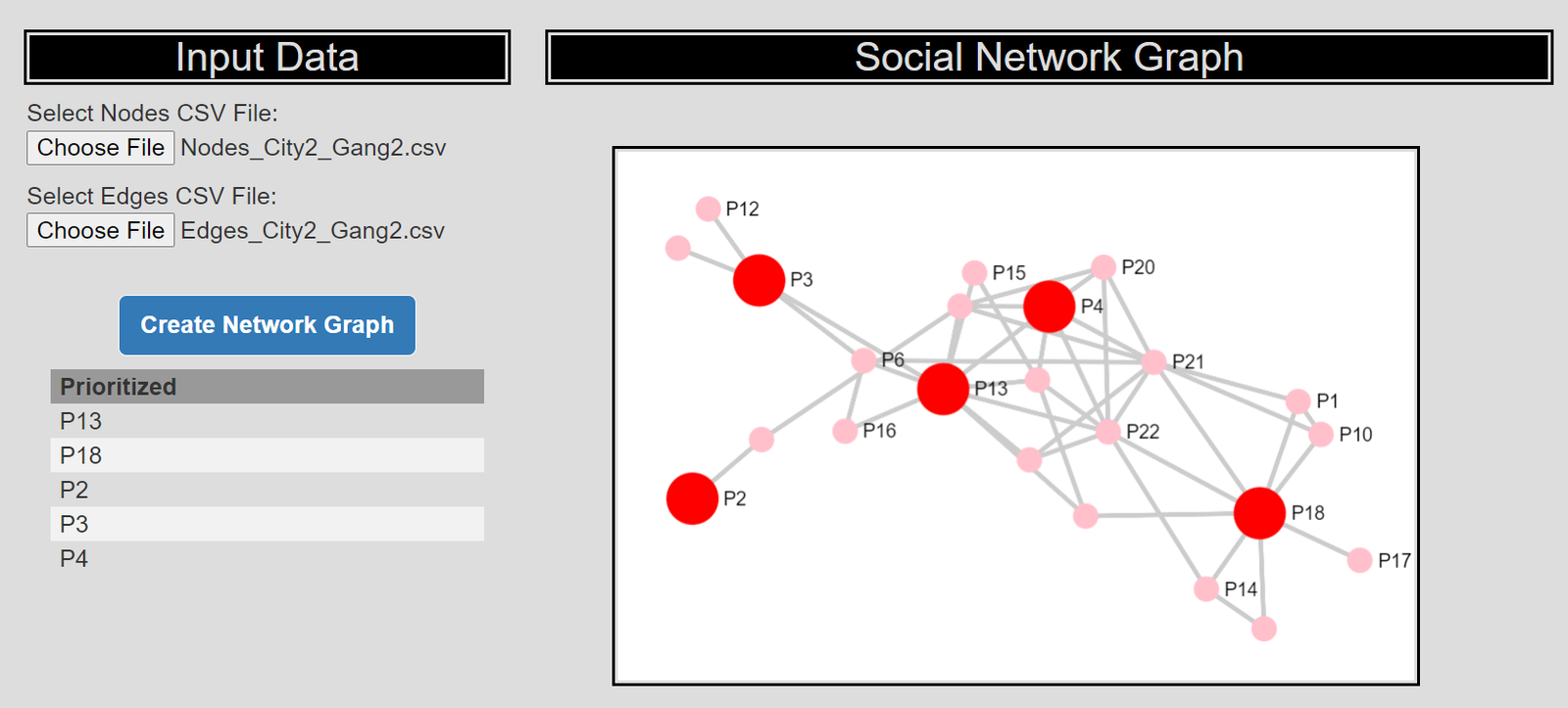
Here I discuss my work on social network algorithms to prioritize individuals to spread the message in a focussed deterrence intervention. This is opposite how many people view “spreading” in a network, I identify something good I want to spread, and seed the network in a way to optimize that spread:

I also have a primer on SNA, which discusses how crime analysts typically define nodes and edges using administrative data.

Listen to the interview as I discuss more general advice – in SNA it matters what you want to accomplish in the end as to how you would define the network. So I discuss how you may want to define edges via victimization to prevent retaliatory violence (I think that would make sense for violence interupptors to be proactive for example).

I also give an example of how detective case allocation may make sense to base on SNA – detectives have background with an individuals network (e.g. have a rapport with a family based on prior cases worked).

28:25 – 33:15, Be proactive as an analyst and learn to code

Here Manny asked the question of how do analysts prevent their role being turned into more administrative role (just get requests and run simple reports). I think the solution to this (not just in crime analysis, but also being an analyst in the private sector) is to be proactive. You shouldn’t wait for someone to ask you for specific information, you need to be defining your own role and conducting analysis on your own.

He also asked about crime analysis being under-used in policing. I think being stronger at computer coding opens up so many opportunities that learning python, R, SQL, is the area I would like to see stronger skills across the industry. And this is a good career investment as it translates to private sector roles.

33:15 – 37:00, How ChatGPT can be used by crime analysts

I discuss how ChatGPT may be used by crime analysis to summarize qualitative incident data and help inform . (Check out this example by Andreas Varotsis for an example.)

To be clear, I think this is possible, but the tech I don’t think is quite up to that standard yet. Also do not submit LEO sensitive data to OpenAI!

Also always feel free to reach out if you want to nerd out on similar crime analysis questions!

Ask me anything: Advice for learning statistics?

For a bit of background, Loki, a computer science student in India, was asking me about my solution to the DrivenData algae bloom competition. Much of our back and forth was specific to my coding solution and “how I knew how to do that” (in particular I used a machine learning variant of doubly robust estimation in part of the solution, which I am sure others have used before but is not real common that I see, it is more often “causal inference” motivated). As for more general advice in learning, I said:

Only advice is to learn stats – not just for competitions but for real-world jobs. Many people are just copy-pasting code, and don’t know what they are doing. Understanding selection bias is important in many real-world scenarios. Often times it is just knowing a little about the scientific scenario you are modeling, and correctly formulating a model.

In response Loki asks:

I decided to take your suggestion and strengthen my grasp on statistics. I consider myself somewhere between beginner to intermediate in stats. I came across several resources on the internet, but feel confused about what to go with. I am wondering if “The Elements of Statistical Learning” by Trevor Hastie and Robert Tibishirani is a good one to start with. Or could you please suggest any books/lectures/courses that have practical applications to solidify my understanding of statistics that you have personally read or liked?

Which I think is a good piece to expand to the readers on my blog in general. Here is my response:

I would not start with that book. It is a mistake to start with too advanced of material. (I don’t learn anything that way anyway.)

Starting from the basics, no joke Gonick’s Cartoon Guide to Statistics is in my opinion the best intro to statistics and probability book. After that, it is important to understand causality – like really understand it – selection bias lurks everywhere. (I am not sure I have great advice for books that focus on causality, Pearl’s book is quite tough, maybe Shadish, Cook, Campbell Experimental and Quasi-Experimental Designs and/or Mostly Harmless Econometrics).

After that, follow questions on https://stats.stackexchange.com, it is high quality on average (many internet sources, like Medium articles or https://datascience.stackexchange.com, are very low quality on average – they can have gems but more often than not they are bad for anything besides copy/pasting code). Andrew Gelman’s blog is another good source for contemporary discussion around stats/research/pitfalls, https://statmodeling.stat.columbia.edu.

In terms of more advanced modeling, after having the basics down, I would suggest Harrell’s Regression Modeling Strategies before the Hastie book. You can interpret pretty much all of machine learning in terms of regression models. For small datasets, understanding how to do simpler regression modeling the right way is the best approach.

When moving onto machine learning, then maybe the Hastie book is a good resource (I didn’t find it all that much useful at this point beyond web resources). Statquest videos are very good walkthroughs of more complicated ML algorithms, https://www.youtube.com/@statquest, trees/boosting/neural-networks.

This is a hodge-podge – I don’t tend to learn things just to learn them – I have a specific project in mind and try to tackle that project the best I can. Many of these resources are items I picked up along the way (Gonick I got to review intro stats books for teaching, Harrell’s I picked up to learn a bit more about non-linear modeling with splines, Statquest I reviewed when interviewing for data science positions).

It is a long road to get to where I am. It was not via picking a book and doing intense study, it was a combination of applied projects and learning new things over time. I learned a crazy lot from the Cross Validated site when I was in grad school. (For those interested in optimization, the Operations Research site is also very high quality.) That was more broad learning though – seeing how people tackled problems in different domains.

Getting access to paywalled newspaper and journal articles

So recently several individuals have asked about obtaining articles they do not have access to that I cite in my blog posts. (Here or on the American Society of Evidence Based Policing.) This is perfectly fine, but I want to share a few tricks I have learned on accessing paywalled newspaper articles and journal articles over the years.

I currently only pay for a physical Sunday newspaper for the Raleigh News & Observer (and get the online content for free because of that). Besides that I have never paid for a newspaper article or a journal article.

Newspaper paywalls

Two techniques for dealing with newspaper paywalls. 1) Some newspapers you get a free number of articles per month. To skirt this, you can open up the article in a private/incognito window on your preferred browser (or open up the article in another browser entirely, e.g. you use Chrome most of the time, but have Firefox just for this on occasion.)

If that does not work, and you have the exact address, you can check the WayBack machine. For example, here is a search for a WaPo article I linked to in last post. This works for very recent articles, so if you can stand being a few days behind, it is often listed on the WayBack machine.

Journal paywalls

Single piece of advice here, use Google Scholar. Here for example is searching for the first Braga POP Criminology article in the last post. Google scholar will tell you if a free pre or post-print URL exists somewhere. See the PDF link on the right here. (You can click around to “All 8 Versions” below the article as well, and that will sometimes lead to other open links as well.)

Quite a few papers have PDFs available, and don’t worry if it is a pre-print, they rarely substance when going into print.1

For my personal papers, I have a google spreadsheet that lists all of the pre-print URLs (as well as the replication materials for those publications).

If those do not work, you can see if your local library has access to the journal, but that is not as likely. And I still have a Uni affiliation that I can use for this (the library and getting some software cheap are the main benefits!). But if you are at that point and need access to a paper I cite, feel free to email and ask for a copy (it is not that much work).

Most academics are happy to know you want to read their work, and so it is nice to be asked to forward a copy of their paper. So feel free to email other academics as well to ask for copies (and slip in a note for them to post their post-prints to let more people have access).

The Criminal Justician and ASEBP

If you like my blog topics, please consider joining the American Society of Evidence Based Policing. To be clear I do not get paid for referrals, I just think it is a worthwhile organization doing good work. I have started a blog series (that you need a membership for to read), and post once a month. The current articles I have written are:

So if you want to read more of my work on criminal justice topics, please join the ASEBP. And it is of course a good networking resource and training center you should be interested in as well.


  1. You can also sign up for email alerts on Google Scholar for papers if you find yourself reading a particular author quite often.↩︎

Random notes, digital art, and pairwise comparisons is polynomial

So not too much in the hopper for the blog at the moment. Have just a bunch of half-baked ideas (random python tips, maybe some crime analysis using osmnx, scraping javascript apps using selenium, normal nerd data science stuff).

Still continuing my blog series on the American Society of Evidence Based Policing, and will have a new post out next week on officer use of force.

If you have any suggestions for topics always feel free to ask me anything!


Working on some random digital art (somewhat focused on maps but not entirely). For other random suggestions I like OptArt and Rick Wicklin’s posts.

Dall-E is impressive, and since it has an explicit goal of creating artwork I think it is a neat idea. Chat bots I have nothing good to say. Computer scientists working on them seem to be under the impression that if you build a large/good enough language model out pops general intelligence. Wee bit skeptical of that.


At work a co-worker was working on timing applications for a particular graph-database/edge-detection project. Initial timings on fake data were not looking so good. Here we have number of nodes and timings for the application:

  Nodes    Minutes
   1000       0.16
  10000       0.25
 100000       1.5
1000000      51

Offhand people often speak about exponential functions (or growth), but here what I expect is we are really looking at is pairwise comparisons (not totally familiar with the tech the other data scientist is using, so I am guessing the algorithmic complexity). So this likely scales something like (where n is the number of nodes in the graph):

Time = Fixed + C1*(n) + C2*(n choose 2) + e

Fixed is just a small constant, C1 is setting up the initial node database, and C2 is the edge detection which I am guessing uses pairwise comparisons, (n choose 2). We can rewrite this to show that the binomial coefficient is really polynomial time (not exponential) in terms of just the number of nodes.

C2*[n choose 2] = C2*[{n*(n-1)}/2]
                  C2*[ (n^2 - n)/2 ]
                  C2/2*[n^2 - n]
                  C2/2*n^2 - C2/2*n

And so we can rewrite our original equation in terms of simply n:

Time = Fixed + (C1 - C2/2)*N + C2/2*N^2

Doing some simple R code, we can estimate our equation:

n <- 10^(3:6)
m <- c(0.16,0.25,1.5,51)
poly_mod <- lm(m ~ n + I(n^2))

Since this fits 3 parameters with only 4 observations, the fit is (not surprisingly) quite good. Which to be clear does not mean much, if really cared would do much more sampling (or read the docs more closely about the underlying tech involved):

> pred <- predict(poly_mod)
> cbind(n,m,pred)
      n     m       pred
1 1e+03  0.16  0.1608911
2 1e+04  0.25  0.2490109
3 1e+05  1.50  1.5000989
4 1e+06 51.00 50.9999991

And if you do instead poly_2 <- lm(m ~ n + choose(n,2)) you get a change in scale of the coefficients, but the same predictions.

We really need this to scale in our application at work to maybe over 100 million records, so what would we predict in terms of minutes based on these initial timings?

> nd = data.frame(n=10^(7:8))
> predict(poly_mod,nd)/60 # convert to hours
         1          2
  70.74835 6934.56850

So doing 10 million records will take a few days, and doing 100 million will be close to 300 days.

With only 4 observations not much to chew over (really it is too few to say it should be a different model). I am wondering though how to best handle errors for these types of extrapolations. Errors are probably not homoskedastic for such timing models (error will be larger for larger number of nodes). Maybe better to use quantile regression (and model the median?). I am not sure (and that advice I think will also apply to modeling exponential growth as well).

Surpassed 100k views in 2022

For the first time, yearly view counts have surpassed 100,000 for my blog.

I typically get a bump of (at best) a few hundred views when I first post a blog. But the most popular posts are all old ones, and I get the majority of my traffic via google searches.

Around March this year monthly bumped up from around 9k to 11k views per month. Not sure of the reason (it is unlikely due to any specific inidividual post, as you can see, none of the most popular posts were posted this year). A significant number of the views are likely bots (what percent overall though I have no clue). So it is possible my blog was scooped up in some other aggregators/scrapers around that time (I would think those would not be counted as search engine referrals though).

One interesting source for the blog, when doing academic style posts with citations, my blog gets picked up by google scholar (see here for example). It is not a big source, but likely a more academic type crowd being referred to the blog (I can tell people have google scholar alerts – when scholar indexes a post I get a handful of referrals).

I have some news coming soon about writing a more regular criminal justice column for an organization (readers will have to wait alittle over a week). But I also do Ask Me Anything, so always feel free to send me an email or comment on here (started AMA as I get a trickle of tech questions via email anyway, and might as well share my response with everyone).

I typically just blog generally about things I am working on. So maybe next up is that auto-ml libraries often have terrible defaults for hypertuning random forests, or maybe an example of data envelopment analysis, or quantile regression for analyzing response times, or monitoring censored data are all random things I have been thinking about recently. But no guarantees about any those topics in particular!

Using weights in regression examples

I have come across several different examples recently where ‘use weights in regression’ was the solution to a particular problem. I will outline four recent examples.

Example 1: Rates in WDD

Sophie Curtis-Ham asks whether I can extend my WDD rate example to using the Poisson regression approach I outline. I spent some time and figured out the answer is yes.

First, if you install my R package ptools, we can use the same example in that blog post showing rates (or as per area, e.g. density) in my internal wdd function using R code (Wheeler & Ratcliffe, 2018):

library(ptools)

crime <- c(207,308,178,150,110,318,157,140)
type <- c('t','ct','d','cd','t','ct','d','cd')
ti <- c(0,0,0,0,1,1,1,1)
ar <- c(1.2,0.9,1.5,1.6,1.2,0.9,1.5,1.6)

df <- data.frame(crime,type,ti,ar)

# The order of my arguments is different than the 
# dataframe setup, hence the c() selections
weight_wdd <- wdd(control=crime[c(2,6)],
                  treated=crime[c(1,5)],
                  disp_control=crime[c(4,8)],
                  disp_treated=crime[c(3,7)],
                  area_weights=ar[c(2,1,4,3)])

# Estimate -91.9 (31.5) for local

So here the ar vector is a set of areas (imagine square miles or square kilometers) for treated/control/displacement/displacementcontrol areas. But it would work the same if you wanted to do person per-capita rates as well.

Note that the note says the estimate for the local effect, in the glm I will show I am just estimating the local, not the displacement effect. At first I tried using an offset, and that did not change the estimate at all:

# Lets do a simpler example with no displacement
df_nod <- df[c(1,2,5,6),]
df_nod['treat'] <- c(1,0,1,0)
df_nod['post'] <- df_nod['ti']

# Attempt 1, using offset
m1 <- glm(crime ~ post + treat + post*treat + offset(log(ar)),
          data=df_nod,
          family=poisson(link="identity"))
summary(m1) # estimate is  -107 (30.7), same as no weights WDD

Maybe to get the correct estimate via the offset approach you need to do some post-hoc weighting, I don’t know. But we can use weights and estimate the rate on the left hand side.

# Attempt 2, estimate rate and use weights
# suppressWarnings is for non-integer notes
df_nod['rate'] <- df_nod['crime']/df_nod['ar']
m2 <- suppressWarnings(glm(rate ~ post + treat + post*treat,
          data=df_nod,
          weights=ar,
          family=poisson(link="identity")))
summary(m2) # estimate is same as no weights WDD, -91.9 (31.5)

The motivation again for the regression approach is to extend the WDD test to scenarios more complicated than simple pre/post, and using rates (e.g. per population or per area) seems to be a pretty simple thing people may want to do!

Example 2: Clustering of Observations

Had a bit of a disagreement at work the other day – statistical models used for inference of coefficients on the right hand side often make the “IID” assumption – independent and identically distributed residuals (or independent observations conditional on the model). This is almost entirely focused on standard errors for right hand side coefficients, when using machine learning models for purely prediction it may not matter at all.

Even if interested in inference, it may be the solution is to simply weight the regression. Consider the most extreme case, we simply double count (or here repeat count observations 100 times over):

# Simulating simple Poisson model
# but replicating data
set.seed(10)
n <- 600
repn <- 100
id <- 1:n
x <- runif(n)
l <- 0.5 + 0.3*x
y <- rpois(n,l)
small_df <- data.frame(y,x,id)
big_df <- data.frame(y=rep(y,repn),x=rep(x,repn),id=rep(id,repn))

# With small data 
mpc <- glm(y ~ x, data=small_df, family=poisson)
summary(mpc)

# Note same coefficients, just SE are too small
mpa <- glm(y ~ x, data=big_df, family=poisson)

vcov(mpc)/vcov(mpa) # ~ 100 times too small

So as expected, the standard errors are 100 times too small. Again this does not cause bias in the equation (and so will not cause bias if the equation is used for predictions). But if you are making inferences for coefficients on the right hand side, this suggests you have way more precision in your estimates than you do in reality. One solution is to simply weight the observations inverse the number of repeats they have:

big_df$w <- 1/repn
mpw <- glm(y ~ x, weight=w, data=big_df, family=poisson)
summary(mpw)
vcov(mpc)/vcov(mpw) # correct covariance estimates

And this will be conservative in many circumstances, if you don’t have perfect replication across observations. Another approach though is to cluster your standard errors, which uses data to estimate the residual autocorrelation inside of your groups.

library(sandwich)
adj_mpa <- vcovCL(mpa,cluster=~id,type="HC2")
vcov(mpc)/adj_mpa   # much closer, still *slightly* too small

I use HC2 here as it uses small sample degree of freedom corrections (Long & Ervin, 2000). There are quite a few different types of cluster corrections. In my simulations HC2 tends to be the “right” choice (likely due to the degree of freedom correction), but I don’t know if that should generally be the default for clustered data, so caveat emptor.

Note again though that the cluster standard error adjustments don’t change the point estimates at all – they simply adjust the covariance matrix estimates for the coefficients on the right hand side.

Example 3: What estimate do you want?

So in the above example, I exactly repeated everyone 100 times. You may have scenarios where you have some observations repeated more times than others. So above if I had one observation repeated 10 times, and another repeated 2 times, the correct weights in that scenario would be 1/10 and 1/2 for each row inside the clusters/repeats. Here is another scenario though where we want to weight up repeat observations though – it just depends on the exact estimate you want.

A questioner wrote in with an example of a discrete choice type set up, but some respondents are repeated in the data (e.g. chose multiple responses). So imagine we have data:

Person,Choice
  1      A  
  1      B  
  1      C  
  2      A  
  3      B  
  4      B  

If you want to know the estimate in this data, “pick a random person-choice, what is the probability of choosing A/B/C?”, the answer is:

A - 2/6
B - 3/6
C - 1/6

But that may not be what you really want, it may be you want “pick a random person, what is the probability that they choose A/B/C?”, so in that scenario the correct estimate would be:

A - 2/4
B - 3/4
C - 1/4

To get this estimate, we should weight up responses! So typically each row would get a weight of 1/nrows, but here we want the weight to be 1/npersons and constant across the dataset.

Person,Choice,OriginalWeight,UpdateWeight
  1      A      1/6             1/4
  1      B      1/6             1/4
  1      C      1/6             1/4
  2      A      1/6             1/4
  3      B      1/6             1/4
  4      B      1/6             1/4

And this extends to whatever regression model if you want to model the choices as a function of additional covariates. So here technically person 1 gets triple the weight of persons 2/3/4, but that is the intended behavior if we want the estimate to be “pick a random person”.

Depending on the scenario you could do two models – one to estimate the number of choices and another to estimate the probability of a specific choice, but most people I imagine are not using such models for predictions so much as they are for inferences on the right hand side (e.g. what influences your choices).

Example 4: Cross-classified data

The last example has to do with observations that are nested within multiple hierarchical groups. One example that comes up in spatial criminology – we want to do analysis of some crime reduction/increase in a buffer around a point of interest, but multiple buffers overlap. A solution is to weight observations by the number of groups they overlap.

For example consider converting incandescent street lamps to LED (Kaplan & Chalfin, 2021). Imagine that we have four street lamps, {c1,c2,t1,t2}. The figure below display these four street lamps; the t street lamps are treated, and the c street lamps are controls. Red plus symbols denote crime locations, and each street lamp has a buffer of 1000 feet. The two not treated circle street lamps overlap, and subsequently a simple buffer would double-count crimes that fall within both of their boundaries.

If one estimated a treatment effect based on these buffer counts, with the naive count within buffer approach, one would have:

c1 = 3    t1 = 1
c2 = 4    t2 = 0

Subsequently an average control would then be 3.5, and the average treated would be 0.5. Subsequently one would have an average treatment effect of 3. This however would be an overestimate due to the overlapping buffers for the control locations. Similar to example 3 it depends on how exactly you want to define the average treatment effect – I think a reasonable definition is simply the global estimate of crimes reduced divided by the total number of treated areas.

To account for this, you can weight individual crimes. Those crimes that are assigned to multiple street lamps only get partial weight – if they overlap two street lamps, the crimes are only given a weight of 0.5, if they overlap three street lamps within a buffer area those crimes are given a weight of 1/3, etc. With such updated weighted crime estimates, one would then have:

c1 = 2    t1 = 1
c2 = 3    t2 = 0

And then one would have an average of 2.5 crimes in the control street lamps, and subsequently would have a treatment effect reduction per average street lamp of 2 crimes overall.

This idea I first saw in Snijders & Bosker (2011), in which they called this cross-classified data. I additionally used this technique with survey data in Wheeler et al. (2020), in which I nested responses in census tracts. Because responses were mapped to intersections, they technically could be inside multiple census tracts (or more specifically I did not know 100% what tract they were in). I talk about this issue in my dissertation a bit with crime data, see pages 90-92 (Wheeler, 2015). In my dissertation using D.C. data, if you aggregated that data to block groups/tracts the misallocation error is likely ~5% in the best case scenario (and depending on data and grouping, could be closer to 50%).

But again I think a reasonable solution is to weight observations, which is not much different to Hipp & Boessan’s (2013) egohoods.

References

Job advice for entry crime analysts

I post occasionally on the Crime Analysis Reddit, and a few recent posts I mentioned about expanding the net to private sector gigs for those interested in crime analysis. And got a question from a recent student as well, so figured a blog post on my advice is in order.

For students interested in crime analysis, it is standard advice to do an internship (while a student), and that gets you a good start on networking. But if that ship has sailed and you are now finished with school and need to get a job that does not help. Also standard to join the IACA (and if you have a local org, like TXLEAN for Texas, you can join that local org and get IACA membership at the same time). They have job boards for openings, and for local it is a good place to network as well for entry level folks. IACA has training material available as well.

Because there are not that many crime analysis jobs, I tell students to widen their net and apply to any job that lists “analyst” in the title. We hire many “business analysts” at Gainwell, and while having a background in healthcare is nice it is not necessary. They mostly do things in Excel, Powerpoint, and maybe some SQL. Probably more have a background in business than healthcare specifically. Feel free to take any background experience in the job description not as requirements but as “nice to have”.

These are pretty much the same data skills people use in crime analysis. So if you can do one you can do the other.

This advice is also true for individuals who are currently crime analysts and wish to pursue other jobs. Unfortunately because crime analysis is more niche in departments, there is not much upward mobility. Other larger organizations that have analysts will just by their nature have more senior positions to work towards over your career. Simultaneously you are likely to have a larger salary in the private sector than public sector for even the same entry level positions.

Don’t get the wrong impression on the technical skills needed for these jobs if you read my blog. Even more advanced data science jobs I am mostly writing python + SQL. I am not writing bespoke optimization functions very often. So in terms of skills for analyst positions I just suggest focusing on Excel. My crime analysis course materials I intentionally did in a way to get you a broad background that is relevant for other analyst positions as well (some SQL/Powerpoint, but mostly Excel).

Sometimes people like to think doing crime analysis is a public service, so look down on going to private sector. Plenty of analysts in banks/healthcare do fraud/waste/abuse that have just as large an impact on the public as do crime analysts, so I think this opinion is misguided in general.

Many jobs at Gainwell get less than 10 applicants. Even if these jobs have listed healthcare background requirements, if they don’t have options among the pool those doing the hiring will lower their expectations. I imagine it is the same for many companies. Just keep applying to analyst jobs and you will land something eventually.

I wish undergrad programs did a better job preparing social science students with tech skills. It is really just minor modifications – courses teaching Excel/SQL (maybe some coding for real go-getters). Better job at making stats relevant to the real world business applications (calculating expected values/variance and trends in those is a common task, doing null hypothesis significance testing is very rare). But you can level up on Excel with various online resources, my course included.