Won NIJ competition on surveys

The submission Gio and myself put together, Using Every Door Direct Mail Web Push Surveys and Multi-level modelling with Post Stratification to estimate Perceptions of Police at Small Geographies, has won the NIJ Innovations in Measuring Community Attitudes Survey challenge.

Specifically we took 1st in the non-probability section of the competition. The paper has the details, but using every door direct mail + post-stratifying the estimates is the approach we advocate. If you are a city or research group interested in implementing this and need help, feel free to get in touch.

Of course if you want to do this yourself go for it (part of the reason it won was because the method should be doable for many agencies in house), but letting me and Gio know we were the inspiration is appreciated!

Second, for recruiting for criminology PhDs, CRIME De-Coder has teamed up with the open access CrimRXiv consortium

This example shows professor adverts, but I think the best value add for this is for more advanced local govt positions. Anymore many of those civil service gigs are very competitive with lagging professor salaries.

For people hiring advanced roles, there are two opportunities. One is advertising – so for about the same amount as advertising on LinkedIn, you can publish a job advert. This is much more targeted than LinkedIn, so if you want PhD talent this is a good deal to get your job posting on the right eyeballs.

The second service is recruiting for a position. This is commission based – if I place a candidate for the role then you pay the recruiter (me and CrimRXiv) a commission. For that I personally reach out to my network of people with PhDs interested in positions, and do the first round of vetting for your role.

Third, over on Crime De-Coder I have another round of the newsletter up, advice this round is that many smaller cities have good up and coming tech markets, plus advice about making fonts larger in python/R plots. (Note in response to that post, Greg Ridgeway says it is better to save as vector graphics as oppossed to high res PNG. Vector is slightly more work to check everything is kosher in the final produced plot, but that is good advice from Greg. I am lazy with the PNG advice.)

No more newsletters this year, but let me know if you want to sign up and I will add you to the list.

Last little tidbit, in the past I have used the pdftk tool to combine multiple PDFs together. This is useful when using other tools to create documents, so you have multiple outputs in the end (like a cover page or tech appendix), and want to combine those all together into a single PDF to share. But one thing I noticed recently, if your PDF has internal table of content (TOC) links (as is the case for LaTeX, or in my case a document built using Quarto), using pdftk will make the TOC links go away. You can however use ghostscript instead, and the links still work as normal.

On my windows machine, it looks something like:

gswin64 -q -sDEVICE=pdfwrite -o MergedDoc.pdf CoverPage.pdf Main.pdf Appendix.pdf

So a few differences that if you just google. Installing the 64 bit version on my windows machine, the executable is gswin64, not gs from the command line. Second, I needed to manually add C:\Program Files\gs\gs10.02.1\bin to my PATH for this to work at the command prompt the way you would expect, installing did not do that directly.

Quarto is awesome by the way – definitely suggest people go check that out.

Sentence embeddings and caching huggingface models in github actions

For updates on Crime De-Coder:

This is actually more born out from demand interacting with crime analysis groups – it doesn’t really make sense for me to swoop in and say “do X/Y/Z, here is my report”. My experience doing that with PDs is not good – my recommendations often do not get implemented. So it is important to upskill your current analysts to be able to conduct more rigorous analysis over time.

Some things it is better to have an external person do the report (such as program evaluation, cost-benefit analysis, or racial bias metrics). But things like generating hotspots and chronic offender lists, those should be something your crime analysis unit learns how to do.

You can of course hire me to do those things, but if you don’t train your local analysts to take over the job, you have to perpetually hire me to do that. Which may make sense for small departments without an internal crime analysis unit. But for large agencies you should be using your crime analysts to do reports like that.


This post, I also wanted to share some work on NLP. I have not been immune at work given all the craze. I am more impressed with vector embeddings and semantic search though than I am with GenAI applications. GenAI I think will be very useful, like a more advanced auto-complete, but I don’t think it will put us all out of work anytime soon.

Vector embeddings, for those not familiar, are taking a text input and turning it into numbers. You can then do nearness calculations with the numbers. So say you had plain text crime narrative notes on modus operandi, and wanted to search “breaking car window and stealing purse” – you don’t want to do an exact search on that phrase, but a search for text that is similar. So the vector similarity search may return a narrative that is “break truck back-window with pipe, take backpack”. Not exactly the same, but semantically very similar.

Sentencetransformers makes this supersimple (no need to use external APIs for this).

from sentence_transformers import SentenceTransformer, util
model = SentenceTransformer('all-MiniLM-L6-v2')

# Base query
query = ['breaking car window and stealing purse']

# Example MO
mo = ['break truck back window with pipe, steal backpack',
      'pushing in a window AC unit, steal TV and sneakers',
      'steal car from cloned fab, joyride']

#Compute embedding for both lists
qemb = model.encode(query, convert_to_tensor=True)
moemb = model.encode(mo, convert_to_tensor=True)

#Compute cosine-similarities
cosine_scores = util.cos_sim(moemb, qemb)
print(cosine_scores)

So you have your query, and often people just return the top-k results, since to know “how close is reasonably close” is difficult in practice (google pretty much always returns some results, even if they are off the mark!).

I am quite impressed with the general models for this (even very idiosyncratic documents and jargon it tends to do quite well). But if you want to embed specifically trained models on different tasks, I often turn to simpletransformers. Here is a model based on clinical case notes.

from simpletransformers.language_representation import RepresentationModel

model = RepresentationModel("bert", "medicalai/ClinicalBERT")
sent1 = ["Procedure X-ray of wrist"] # needs to be a list
wv1 = model.encode_sentences(sent1, combine_strategy="mean")

For another example, I shared a github repo, hugging_cache, where I did some work on how to cache huggingface models in a github actions script. This is useful for unit tests, so you don’t need to redownload the model everytime.

Github cache size for free accounts is 10 gigs (and you need the environment itself, which is a few gigs). So huggingface models up to say around 4 (maybe 5) gigs will work out OK in this workflow. So not quite up to par with the big llama models, but plenty large enough for these smaller embedding models.

It is not very difficult to build a local, in-memory vector search database. Which will be sufficient for many individuals. So a crime analyst could build a local search engine for use – redo vector DB on a batch job, then just have a tool/server to do the local lookup. (Or just use a local sqlite database is probably sufficient for a half dozen analysts/detectives may use this tool every now and then.)

Forecasts need to have error bars

Richard Rosenfeld in the most recent Criminologist published a piece about forecasting national level crime rates. People complain about the FBI releasing crime stats a year late, academics are worse; Richard provided “forecasts” for 2021 through 2025 for an article published in late 2023.

Even ignoring the stalecasts that Richard provided – these forecasts had/have no chance of being correct. Point forecasts will always be wrong – a more reasonable approach is to provide the prediction intervals for the forecasts. Showing error intervals around the forecasts will show how Richard interpreting minor trends is likely to be misleading.

Here I provide some analysis using ARIMA models (in python), to illustrate what reasonable forecast error looks like in this scenario, code and data on github.

You can get the dataset on github, but just some upfront with loading the libraries I need and getting the data in the right format:

import pandas as pd
from statsmodels.tsa.arima.model import ARIMA
import matplotlib.pyplot as plt

# via https://www.disastercenter.com/crime/uscrime.htm
ucr = pd.read_csv('UCR_1960_2019.csv')
ucr['VRate'] = (ucr['Violent']/ucr['Population'])*100000
ucr['PRate'] = (ucr['Property']/ucr['Population'])*100000
ucr = ucr[['Year','VRate','PRate']]

# adding in more recent years via https://cde.ucr.cjis.gov/LATEST/webapp/#/pages/docApi
# I should use original from counts/pop, I don't know where to find those though
y = [2020,2021,2022]
v = [398.5,387,380.7]
p = [1958.2,1832.3,1954.4]
ucr_new = pd.DataFrame(zip(y,v,p),columns = list(ucr))
ucr = pd.concat([ucr,ucr_new],axis=0)
ucr.index = pd.period_range(start='1960',end='2022',freq='A')

# Richard fits the model for 1960 through 2015
train = ucr.loc[ucr['Year'] <= 2015,'VRate']

Now we are ready to fit our models. To make it as close to apples-to-apples as Richard’s paper, I just fit an ARIMA(1,1,2) model – I do not do a grid search for the best fitting model (also Richard states he has exogenous factors for inflation in the model, which I do not here). Note Richard says he fits an ARIMA(1,0,2) for the violent crime rates in the paper, but he also says he differenced the data, which is an ARIMA(1,1,2) model:

# Not sure if Richard's model had a trend term, here no trend
violent = ARIMA(train,order=(1,1,2),trend='n').fit()
violent.summary()

This produces the output:

                               SARIMAX Results
==============================================================================
Dep. Variable:                  VRate   No. Observations:                   56
Model:                 ARIMA(1, 1, 2)   Log Likelihood                -242.947
Date:                Sun, 19 Nov 2023   AIC                            493.893
Time:                        19:33:53   BIC                            501.923
Sample:                    12-31-1960   HQIC                           496.998
                         - 12-31-2015
Covariance Type:                  opg
==============================================================================
                 coef    std err          z      P>|z|      [0.025      0.975]
------------------------------------------------------------------------------
ar.L1         -0.4545      0.169     -2.688      0.007      -0.786      -0.123
ma.L1          1.1969      0.131      9.132      0.000       0.940       1.454
ma.L2          0.7136      0.100      7.162      0.000       0.518       0.909
sigma2       392.5640    104.764      3.747      0.000     187.230     597.898
===================================================================================
Ljung-Box (L1) (Q):                   0.13   Jarque-Bera (JB):                 0.82
Prob(Q):                              0.72   Prob(JB):                         0.67
Heteroskedasticity (H):               0.56   Skew:                            -0.06
Prob(H) (two-sided):                  0.23   Kurtosis:                         2.42
===================================================================================

So some potential evidence of over-differencing (with the negative AR(1) coefficient). Looking at violent.test_serial_correlation('ljungbox') there is no significant serial auto-correlation in the residuals. One could use some sort of auto-arima approach to pick a “better” model (it clearly needs to be differenced at least once, also maybe should also be modeling the logged rate). But there is not much to squeeze out of this – pretty much all of the ARIMA models will produce very similar forecasts (and error intervals).

So in the statsmodels package, you can append new data and do one step ahead forecasts, so this is comparable to Richard’s out of sample one step ahead forecasts in the paper for 2016 through 2020:

# To make it apples to apples, only appending through 2020
av = (ucr['Year'] > 2015) & (ucr['Year'] <= 2020)
violent = violent.append(ucr.loc[av,'VRate'], refit=False)

# Now can show insample predictions and forecasts
forecast = violent.get_prediction('2016','2025').summary_frame(alpha=0.05)

If you print(forecast) below are the results. One of the things I want to note is that if you do one-step-ahead forecasts, here the years 2016 through 2020, the standad error is under 20 (this is well within Richard’s guesstimate to be useful it needs to be under 10% absolute error). When you start forecasting multiple years ahead though, the error compounds over time. So to forecast 2022, you need a forecast of 2021. To forecast 2023, you need to forecast 21,22 and then 23, etc.

VRate        mean    mean_se  mean_ci_lower  mean_ci_upper
2016   397.743461  19.813228     358.910247     436.576675
2017   402.850827  19.813228     364.017613     441.684041
2018   386.346157  19.813228     347.512943     425.179371
2019   379.315712  19.813228     340.482498     418.148926
2020   379.210158  19.813228     340.376944     418.043372
2021   412.990860  19.813228     374.157646     451.824074
2022   420.169314  39.803285     342.156309     498.182318
2023   416.906654  57.846105     303.530373     530.282936
2024   418.389557  69.535174     282.103120     554.675994
2025   417.715567  80.282625     260.364513     575.066620

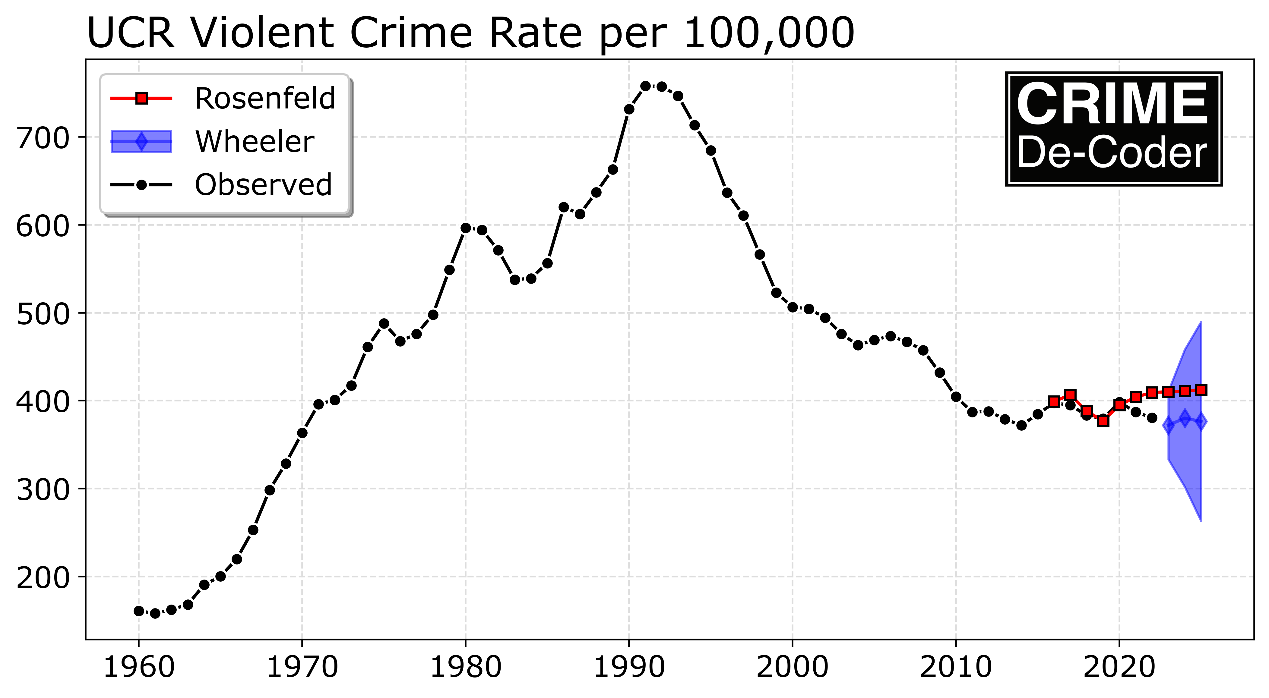
The standard error scales pretty much like sqrt(steps*se^2) (it is additive in the variance). Richard’s forecasts do better than mine for some of the point estimates, but they are similar overall:

# Richard's estimates
forecast['Rosenfeld'] = [399.0,406.8,388.0,377.0,394.9] + [404.1,409.3,410.2,411.0,412.4]
forecast['Observed'] = ucr['VRate']

forecast['MAPE_Andy'] = 100*(forecast['mean'] - forecast['Observed'])/forecast['Observed']
forecast['MAPE_Rick'] = 100*(forecast['Rosenfeld'] - forecast['Observed'])/forecast['Observed']

And this now shows for each of the models:

VRate        mean  mean_ci_lower  mean_ci_upper  Rosenfeld    Observed  MAPE_Andy  MAPE_Rick
2016   397.743461     358.910247     436.576675      399.0  397.520843   0.056002   0.372095
2017   402.850827     364.017613     441.684041      406.8  394.859716   2.023785   3.023931
2018   386.346157     347.512943     425.179371      388.0  383.362999   0.778155   1.209559
2019   379.315712     340.482498     418.148926      377.0  379.421097  -0.027775  -0.638103
2020   379.210158     340.376944     418.043372      394.9  398.500000  -4.840613  -0.903388
2021   412.990860     374.157646     451.824074      404.1  387.000000   6.715985   4.418605
2022   420.169314     342.156309     498.182318      409.3  380.700000  10.367563   7.512477
2023   416.906654     303.530373     530.282936      410.2         NaN        NaN        NaN
2024   418.389557     282.103120     554.675994      411.0         NaN        NaN        NaN
2025   417.715567     260.364513     575.066620      412.4         NaN        NaN        NaN

So MAPE in the held out sample does worse than Rick’s models for the point estimates, but look at my prediction intervals – the observed values are still totally consistent with the model I have estimated here. Since this is a blog and I don’t need to wait for peer review, I can however update my forecasts given more recent data.

# Given updated data until end of series, lets do 23/24/25
violent = violent.append(ucr.loc[ucr['Year'] > 2020,'VRate'], refit=False)
updated_forecast = violent.get_forecast(3).summary_frame(alpha=0.05)

And here are my predictions:

VRate        mean    mean_se  mean_ci_lower  mean_ci_upper
2023   371.977798  19.813228     333.144584     410.811012
2024   380.092102  39.803285     302.079097     458.105106
2025   376.404091  57.846105     263.027810     489.780373

You really need to graph these out to get a sense of the magnitude of the errors:

Note how Richard’s 2021 and 2022 forecasts and general increasing trend have already been proven to be wrong. But it really doesn’t matter – any reasonable model that admitted uncertainty would never let one reasonably interpret minor trends over time in the way Richard did in the criminologist article to begin with (forecasts for ARIMA models are essentially mean-reverting, they will just trend to a mean term in a short number of steps). Richard including exogenous factors actually makes this worse – as you need to forecast inflation and take that forecast error into account for any multiple year out forecast.

Richard has consistently in his career overfit models and subsequently interpreted the tea leaves in various macro level correlations (Rosenfeld, 2018). His current theory of inflation and crime is no different. I agree that forecasting is the way to validate criminological theories – picking up a new pet theory every time you are proven wrong though I don’t believe will result in any substantive progress in criminology. Most of the short term trends criminologists interpret are simply due to normal volatility in the models over time (Yim et al., 2020). David McDowall has a recent article that is much more measured about our cumulative knowledge of macro level crime rate trends – and how they can be potentially related to different criminological theories (McDowall, 2023). Matt Ashby has a paper that compares typical errors for city level forecasts – forecasting several years out tends to product quite inaccurate estimates, quite a bit larger than Richard’s 10% is useful threshold (Ashby, 2023).

Final point that I want to make is that honestly it doesn’t even matter. Richard can continue to keep making dramatic errors in macro level forecasts – it doesn’t matter if he publishes estimates that are two+ years old and already wrong before they go into print. Because unlike what Richard says – national, macro level violent crime forecasts do not help policy response – why would Pittsburgh care about the national level crime forecast? They should not. It does not matter if we fit models that are more accurate than 5% (or 1%, or whatever), they are not helpful to folks on the hill. No one is sitting in the COPS office and is like “hmm, two years from now violent crime rates are going up by 10, lets fund 1342 more officers to help with that”.

Richard can’t have skin the game for his perpetual wrong macro level crime forecasts – there is no skin to have. I am a nerd so I like looking at numbers and fitting models (or here it is more like that XKCD comic of yelling at people on the internet). I don’t need to make up fairy tale hypothetical “policy” applications for the forecasts though.

If you want a real application of crime forecasts, I have estimated for cities that adding an additional home or apartment unit increases the number of calls per service by about 1 per year. So for growing cities that are increasing in size, that is the way I suggest to make longer term allocation plans to increase police staffing to increase demand.

References

Fitting beta binomial in python, Poisson scan stat in R

Sharing two pieces of code I worked on recently for various projects. First is fitting a beta binomial distribution in scipy. I had a need for this the other day, looking at the count of near duplicates in surveys. In that code I just used the method of moments estimator (which can often misbehave).

The top google results for this are all very bad (either code that does not work, or alternatives that are not good advice). One of the articles was even auto-generated content (ala ChatGPT type stuff), that had a few off the mark points (although was superficially what the python solution should look like, so the unwary would be led down a wrong path).

So here I show how to estimate the maximum likelihood estimate for the beta binomial distribution. First, because scipy already has a function for the pmf for the beta-binomial distribution it is pretty simple. For all of the discrete distributions, it should look like -dist.logpmf(..data..,...params...).sum(). In complicated stats speak this is “the negative of the sum of the log likelihood”. It is easier for me anyway to think in terms of the PDF/PMF though (the probability of observing your data given fixed parameters). And you find the parameters that maximize that probability over your entire sample. But to make the math easier we take the logs of the probabilities (so we can work with sums instead of multiplications), the log PMF here, and we take the negative so we find the minimum of the function.

Then you just pass the appropriate arguments to minimize and you are good to go.

import numpy as np
from scipy.optimize import minimize
from scipy.stats import betabinom
np.random.seed(10)

# simulating some random data
a = 0.8
b = 1.2

sim_size = 1000

n = 90
r = betabinom.rvs(n, a, b, size=sim_size)

# minimize negative log likelihood
def bbll(parms,k,n):
    alpha, beta = parms
    ll = betabinom.logpmf(k,n,alpha,beta)
    return -ll.sum()

result = minimize(bbll,[1,1],args=(r,90),method='Nelder-Mead')
print(result.x) # [alpha, beta]

And this returns for me:

>>> print(result.x)
[0.77065051 1.16323611]

Using simple simulations you can often get a feel for different estimators. Here n and sim_size make a decent difference for estimating beta, and beta I think tends to be biased downward in the smaller sample scenarios. (People don’t realize, for these non-normal distributions it is not un-common to need 1000+ observations to get decent un-biased estimates depending on the distribution.)

Note the nature of the data here, it is something like hits [5,8,9], and then a second either constant for every number (if the denominator is say 10 for all the observations, can just pass a constant 10). The denominator can however be variable in this set up, so you could have a set of different denominators like [6,8,10].

a = 1.5
b = 4.1

n = np.random.choice(range(30,90),size=sim_size)
r = betabinom.rvs(n, a, b, size=sim_size)

result = minimize(bbll,[1,1],args=(r,n),method='Nelder-Mead')
print(result.x)

Which returns:

>>> print(result.x)
[1.50563582 3.99837155]

I note here that some examples of beta-binomial use weighted data (the wikipedia page does this). These functions expect unweighted data. Functions that need to be repeatedly called (like the likelihood function here) I don’t like making them general with ifs and other junk, I would rewrite the bbll function for different forms of data and call that different function.

Also, as always, you need to check these to make sure the fitted parameters make sense and reasonably fit your data (plot the predicted PMF vs the observed histogram). The function here can converge, but could converge to non-sense (you probably don’t need to worry about constraints on the parameters, but better starting values are probably a good idea).

For future notes for myself, Guimaraes (2005) has examples of using fixed effects negative binomial and translating to beta-binomial (for fixed n). Also Young-Xu & Chan (2008) is a very nice reference (has Hessian, so if I wanted to estimate standard errors), as well as discussion of determining whether to use this model or a binomial with no extra dispersion.


The second thing I will post about is a scan statistic. The background is imagine someone comes to you and says “Hey, there were 10 robberies in the past week, is that normal or low?”. In the scenario where you have fixed time intervals, e.g. Monday through Sunday, and your data is approximately Poisson distributed, you can calculate the CDF. So say your mean per week over 2 years is 3.1, the probability of observing a count of 10 or more in a specific week is:

> # R code
> 1 - ppois(10-1,3.1)
> [1] 0.001400924

So alittle more than 1 in 1000. But if you ask the question “What is the probability of observing a single week of 10 or more, when I have been monitoring the series for 2 years”, with 52 weeks per year. You would adjust the probability for monitoring the trends for multiple weeks over time:

> p <- ppois(10-1,3.1)
> 1 - p^(52*2)
> [1] 0.1356679

So the probability of observing 10 or more in a single week over a 2 year period is closer to 14%. This multiple comparison issue is more extreme when you consider a sliding window – so can count events that occur in a span of a week, but not all necessarily in your pre-specified Monday to Sunday time period. So maybe you observed 10 in a week span that goes from Wednesday to Tuesday. What is the probability of observing 10 in that ad-hoc week time period over the 3 year monitoring period? This often comes up in news articles, see this post by David Spiegelhalter on pedestrian deaths for an example.

I have added in the Naus (1982) approximate statistic to calculate this in my ptools R package – scanw. If you install the latest version of ptools from github you can run for yourself:

> # R code
> library(devtools)
> install_github("apwheele/ptools") # get most recent
> library(ptools)
>
> # example given above
> scanw(52*2,1,3.1,10)

Which prints out [1] 0.5221948. So adding in the sliding window considerably ups the probability of observing a large clump of events.

I don’t think this is so useful from a crime analyst perspective, moreso from a journalistic perspective ‘oh we saw this number recently, is that anomalous’. If you are actively monitoring crime stats I would suggest you use the stats I describe in Wheeler (2016) to identify current outliers given fixed time intervals from the start. (And this approximation is for Poisson data. Overdispersed will have a higher probability.)

And for reference as well, Prieto-Curiel et al. (2023) have an approach that examines the cumulative sum. I’ve debated on doing that in a control chart style framework as well, but instead of just cumsum(counts), do cumsum(counts - expected). I don’t know how people effectively reset the cumulative charts though and effectively deal with seasonality.

I think my approach in Wheeler (2016) is better to identify anomalous trends right now, the Prieto-Curiel approach is still examining historical data and looking for breaks.

References

Survey duplicates and other stuff

So for various updates. First, I have started an AltAc newsletter, see the first email here. It will be examples of jobs, highlights of criminologists who are in the private sector, and random beginner tech advice (this week was getting started in NLP using simpletransformers, next week I will give a bit of SQL). Email me if you want to be added to the list (open to whomever).

Second, over on CRIME De-Coder I have a post on more common examples of NLP in crime analysis: named entity recognition, semantic similarity, and supervised learning. I have been on an NLP kick lately – everyone thinks genAI (e.g. ChatGPT) is all the rage, most applications though really don’t want genAI, they just think genAI is cool.

Third, Andrew Gelman blogged about the Hogan/Kaplan back and forth. I do like Gelman’s hot takes, even if he is not super in-the-know on current flavors of different micro-econ identification strategies.

Fourth, I have pushed mine and Gio’s whitepaper on using every door direct mail and web based push surveys + MRP to CrimRXiv. Using Every Door Direct Mail Web Push Surveys and Multi-level modelling with Post Stratification to estimate Perceptions of Police at Small Geographies (Circo & Wheeler, 2023). This is our solution to measuring spatially varying attitudes towards police with a reasonable budget (the NIJ community perceptions challenge). Check it out and get in touch if you want to deploy something like that to your jurisdiction.

For a bit of background, we (me and Gio) intentionally did not submit to the other categories in the competition. I don’t think you can reasonably measure micro place community attitudes using any of the other methods in the competition (with the exception of boots on the ground survey takers, which is cost prohibitive and a non-starter for most cities). So we could be like ‘uSiNG TwiTTeR aNd SenTimeNT aNalYSis tO mEasUre HoW mUCh PeoPLe hAtE pOLIcE’, but this is bad both from a measure perspective (sentiment analyses are not good, even ignoring selection biases in those public social media sources) and a tieing it to a particular spatial area perspective. The tieing it to a small spatial area also makes me very hesitant to suggest purely web based adverts to generate survey responses.

Analyzing Survey Duplicates

The last, and biggest thing I wanted to share. Jake Day and Jon Brauer’s blog, Reluctant Criminologists, has a series of posts on analyzing near survey duplicates (also with contribution by Maja Kotlaja). Apparently there was a group with SurveyMonkey/Princeton that gives a recommendation that matches over 85% are cause for concern – so if you take two survey responses, and those two responses have over 85% of the same survey responses, that is symptomatic of fraud in the SurveyMonkey advice.

This is theoretically caused by a malicious actor (such as a survey taker not wanting to do work). So they take an existing survey, duplicate it, but to be sneaky change a few responses to make it look less suspicious (this is not about making up responses whole cloth).

The 85% rule is bad advice and will result in chasing the noise. Many real world criminology surveys will have more random matches, so people will falsely assume surveys are fraudulent. RC do EDA on one of their own surveys and say why they don’t think the over 85% is likely to be fraudulent. (And sign up for their blog and other work while you go check out their post.)

So I give python code how I would analyze survey duplicates, taking into account the nature of the baseline data, Survey Forensics: Identifying Near Duplicate Responses. I show in simulations how you can get more than 85% duplicate matches, even in random data, depending on the marginal distribution of the survey responses.

I also show how to use statistics to identify outliers use false discovery rate corrections, and then cluster like responses together for easier analysis of the identified problem responses. Using data in Raleigh, I show a several groups of outlying survey near duplicates are people just doing run responses (all 5s, 4s, or missings). But I do identify 3 pairs that are somewhat suspicious.

While this is particular type of fraud is not so much a problem in web based surveys, it is not totally irrelevant – you can have people retake web based push surveys by accident. Urban talks about this in terms of analyzing IP addresses. Cell phones and WiFi though some of those could slip through, so this is idea is not totally irrelevant even for web surveys. And for shared WiFi (universities, or people in the same home/apt taking the survey) IP addresses won’t necessarily discriminate.

References

Synthetic control in python: Opioid death increases in Oregon and Washington

So Charles Fain Lehman has a recent post on how decriminalization of opioids in Oregon and Washington (in the name of harm reduction) appear to have resulted in increased overdose deaths. Two recent papers, both using synthetic controls, have come to different conclusions, with Joshi et al. (2023) having null results, and Spencer (2023) having significant results.

I have been doing synth analyses for several groups recently, have published some on micro-synth in the past (Piza et al., 2020). The more I do, the more I am concerned about the default methods. Three main points to discuss here:

  • I think the default synth fitting mechanism is not so great, so I have suggested using Lasso regression (if you want a “real” peer-reviewed citation, check out DeBiasi & Circo (2021) for an application of this technique). Also see this post on crime counts/rates and synth problems, which using an intercept in a Lasso regression avoids.
  • The fitting mechanism + placebo approach to generate inference can be very noisy, resulting in low powered state level designs. Hence I suggest a conformal inference approach to generate the null distribution
  • You should be looking at cumulative effects, not just instant effects in these designs.

I have posted code on Github, and you can see the notebook with the results. I will walk through here quickly. I initially mentioned this technique is a blog post a few years ago (with R code). Here I spent some time to script it up in python.

So first, we load in the data, and go on to conduct the Oregon analysis (you drop Washington as a potential control). Now, a difference in the Abadie estimator (just a stochastic gradient descent optimizer with hard constraints), vs a lasso estimator (soft constraints), is that you need to specify how much to penalize the coefficients. There is no good default for how much, it depends on the scale of your data (doing death rates per 1,000,000 vs per 100,000 will change the amount of penalization), how many rows of data you have, and have many predictor variables you have. So I use an approach to suggest the alpha coefficient for the penalization in a seperate step:

import LassoSynth
import pandas as pd

opioid = pd.read_csv('OpioidDeathRates.csv')
wide = LassoSynth.prep_longdata(opioid,'Period','Rate','State')

# Oregon Analysis
or_data = wide.drop('Washington', axis=1)
oregon = LassoSynth.Synth(or_data,'Oregon',38)

oregon.suggest_alpha() # default alpha is 1

This ends up suggesting an alpha value of 0.17 (instead of default 1). Now you can fit (I passed in the data already to prep it for synth on the init, so no need to re-submit the data):

oregon.fit()
oregon.weights_table()

The fit prints out some metrics, root mean square error and R-squared, {'RMSE': 0.11589514406988406, 'RSquare': 0.7555976595776881}, here for this data. Which offhand looks pretty similar to the other papers (including Charles). And for the weights table, Oregon ends up being very sparse, just DC and West Virginia for controls (plus the intercept):

Group                       Coef
Intercept               0.156239
West Virginia           0.122256
District of Columbia    0.027378

The Lasso model here does constrain the coefficients to be positive, but does not force them to sum to 1 (plus it has an intercept). I think these are all good things (based on personal experience fitting functions). We can graph the fit for the historical data, plus the standard error of the lasso counterfactual forecasts in the post period:

# Default alpha level is 95% prediction intervals for counterfactual
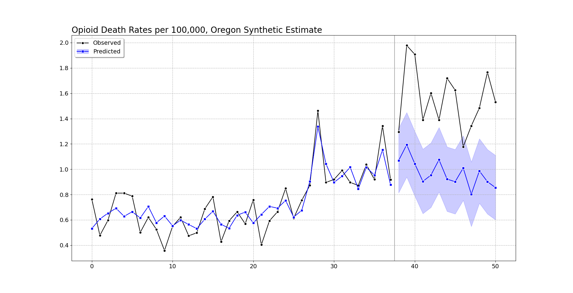
oregon.graph('Opioid Death Rates per 100,000, Oregon Synthetic Estimate')

So you can see the pre-intervention fit is smoother than the monthly data in Oregon, but by eye seems quite reasonable (matches the recent increase and spikes post period 20, starts in Jan-2018, so starting in August-2019). (Perfect fits are good evidence of over-fitting in machine learning.)

Post intervention, after period 37, I do my graph a bit differently. Sometimes people are confused when the intervention starts in the graph, so here I literally split pre/post data lines, so there should be no confusion. I use the conformal inference approach to generate 95% prediction intervals around the counterfactual trend. You can see the counterfactual trend has slightly decreased, whereas Oregon increased and is volatile. Some of the periods are covered by the upper most intervals, but the majority are clearly outside.

Now, besides the fitting function, one point I want to make is people should be looking at cumulative effects, not just instant effects. So Abadie has a global test, using placebos, that looks at the ratio of the pre-fit to post fit (squared errors), then does the placebo p-value based on that stat. This doesn’t have any consideration though for consistent above/below effects.

So pretend the Oregon observed was always within the 95% counterfactual error bar, but was always consistently at the top, around 0.1 increase in overdose deaths. Any single point-wise monthly inference fails to reject the null, but that overall always high pattern is not regular. You want to look at the entire curve, not just a single point. Random data won’t always be high or low, it should fluctuate around the counterfactual estimate.

To do this you look at the cumulative differences between the counterfactual and the observed (and take into account the error distribution for the counterfactuals).

# again default is 95% prediction intervals
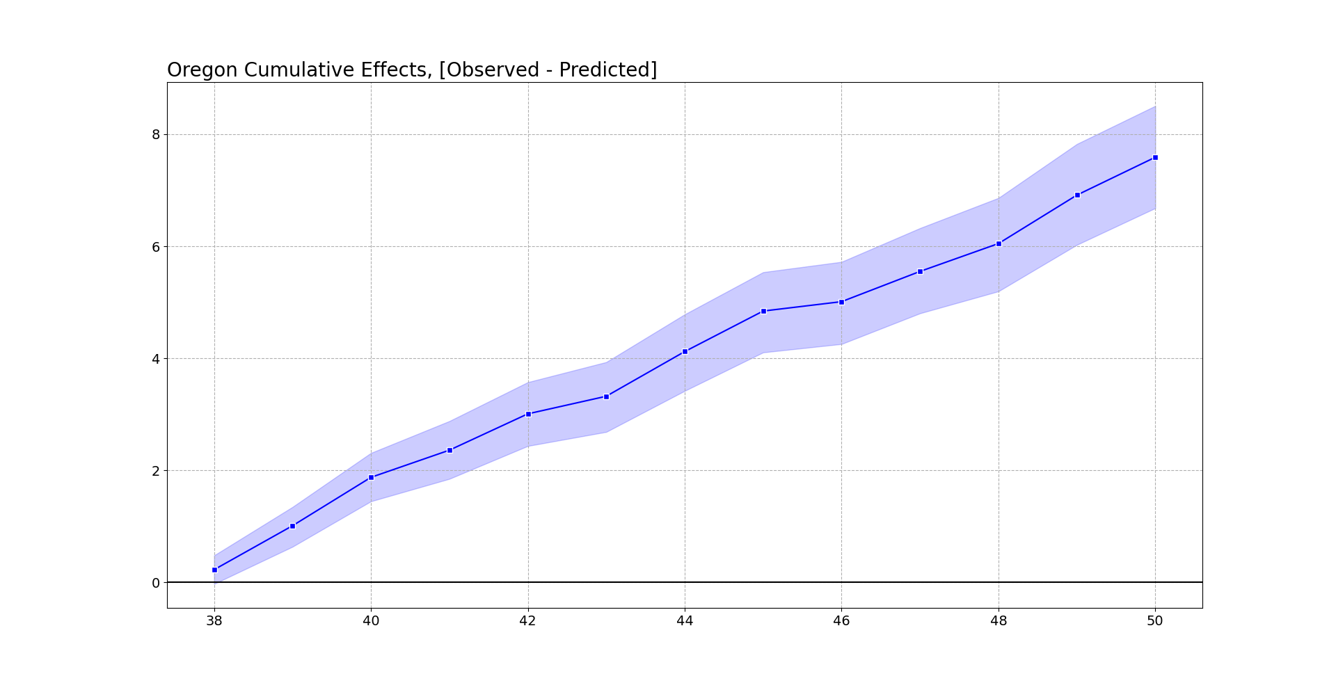
oregon.cumgraph('Oregon Cumulative Effects, [Observed - Predicted]')

Accumulated over time, this is a total of over 7 per 100,000. With Oregon having a population of around 4.1 million, I estimate that the cumulative increased number of overdose deaths is around 290 in Oregon. This is pretty consistent with the results in Spencer (2023) as well (182 increased deaths over fewer months).

To do a global test with this approach, you just look at the very final time period and whether it covers 0. This is what I suggest in-place of the Abadie permutation test, as this has a point estimate and standard error, not just a discrete p-value.

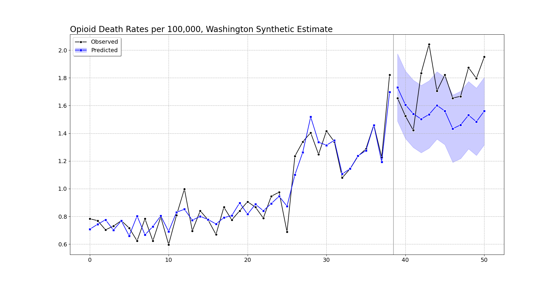
We can do the same analysis for Washington as we did for Oregon. It shows increases, but many of the time periods are covered by the counter-factual 95% prediction interval.

But like I mentioned before, they are consistently high. So when you do the cumulative effects for Washington, they more clearly show increases over time (this data last date is March 2022).

At an accumulated 2.5 per 100,000, with a state population of around 7.7 million, it is around 190 additional overdose deaths in Washington. You can check out the notebook for more stats, Washington has a smaller suggested alpha, so the matched weights have several more states. But the pre-fit is better, and so it has smaller counterfactual intervals. All again good things compared to the default (placebo approach Washington/Oregon will pretty much have the same error distribution, so Washington being less volatile does not matter using that technique).

I get that Abadie is an MIT professor, published a bunch in JASA and well known econ journals, and that his approach is standard in how people do synthetic control analyses. My experience though over time has made me think the default approaches here are not very good – and the placebo approach where you fit many alternative analyses just compounds the issue. (If the fit is bad, it makes the placebo results more variable, causing outlier placebos. People don’t go and do a deep dive of the 49 placebos though to make sure they are well behaved.)

The lasso + conformal approach is how I would approach the problem from my experience fitting machine learning models. I can’t give perfect proof this is a better technique than the SGD + placebo approach by Adadie, but I can release code to at least make it easier for folks to use this technique.

References

  • De Biasi, A., & Circo, G. (2021). Capturing crime at the micro-place: a spatial approach to inform buffer size. Journal of Quantitative Criminology, 37, 393-418.

  • Joshi, S., Rivera, B. D., Cerdá, M., Guy, G. P., Strahan, A., Wheelock, H., & Davis, C. S. (2023). One-year association of drug possession law change with fatal drug overdose in Oregon and Washington. JAMA Psychiatry Online First.

  • Piza, E. L., Wheeler, A. P., Connealy, N. T., & Feng, S. Q. (2020). Crime control effects of a police substation within a business improvement district: A quasi‐experimental synthetic control evaluation. Criminology & Public Policy, 19(2), 653-684.

  • Spencer, N. (2023). Does drug decriminalization increase unintentional drug overdose deaths?: Early evidence from Oregon Measure 110. Journal of Health Economics, 91, 102798.

Soft launching tech recruiting

I am soft-launching a tech recruiting service. I have had conversations with people on all sides of the equation on a regular basis, so I might as well make it a formal thing I do.

If you are an agency looking to fill a role, get in touch. If you are looking for a role, get in touch at https://crimede-coder.com/contact or send an email directly to andrew.wheeler@crimede-coder.com.

Why am I doing this?

I have a discussion with either a friend or second-degree friend about once a month who are current professors who ask me about making the jump to private sector. You can read my post, Make More Money, how I think many criminal justice professors are grossly underpaid. For PhD students you can see my advice at Flipping a CJ PhD to an Alt-Academic career.

If you are a current student or professor and want to chat, reach out and let me know you are interested. I am just going to start keeping a list of folks to help match them to current opportunities.

I have discussions with people who are trying to hire for jobs regularly as well. This includes police departments that are upping their game to hire more advanced roles, think tanks who want to hire early career individuals, and some tech companies in the CJ space who need to fill data science roles.

These are good jobs, and we have good people, so why are these agencies and businesses having a hard time filling these roles? Part of it is advertisement – these agencies don’t do a good job of getting the word out to the right audience. A second part is people have way off-base salary expectations (this is more common for academic positions, post docs I am looking at you). Part of the salary discussion is right sizing the role and expectations – you can’t ask for 10+ years experience and have a 90k salary for someone with an advanced degree – doesn’t really matter what job title you are hiring for.

I can help with both of those obviously – domain knowledge and my network can help your agency right size and fill that role.

Finally, I get cold messaged by recruiters multiple times a month. The straw to finally put this all on paper is I routinely encounter gross incompetence from recruiters. They do not understand the role the business is hiring for, they do not have expertise to evaluate potential candidates, and by cold emailing they clearly do not have a good network to pull potential candidates from.

If you are an agency or company whom you think my network of scholars can help fill your roll get in touch. I only get paid when you fill the position, so it is no cost to try to use my recruiting services. Again will help go over the role with you and say whether it feasible to fill that position as is, or whether it should be tweaked.

Below is my more detailed advice for job seekers. Again reach out if you are a job seeker, even if we have not met we can chat, I will see you do good work, and I will put you on my list of potential applicants to pull from in the future.

Tech Job Applying Advice, P1 Tech Roles

Here is an in-depth piece of advice I gave a friend recently – I think this will be useful in general to individuals in the social sciences who are interested in making the jump to the private sector.

First is understanding what jobs are available. This blog has a focus on quantitative work, but even if you do qualitative work there are tech opportunities. Also some jobs only need basic quant skills (Business Analyst) that any PhD will have (if you know how to use Excel and PowerPoint you have the necessary tech skills to be a business analyst).

Job labels and responsibilities are fuzzy, but here is a rundown of different tech roles and some descriptions:

  • Data Scientist
    • Role, fitting models and automating processes (writing code to shift data around)
    • need to have more advanced coding/machine learning background, e.g. have examples in python/R/SQL and know machine learning concepts
  • Business Analyst
    • anyone with a PhD can do this, Excel/Powerpoint
    • domain knowledge is helpful (which can be learned)
  • Program Manager/Project Manager
    • Help manage teams, roles are similar to “managing grants”, “supervising students”
    • often overlap with various project management strategies (agile, scrum).
    • These names are all stupid though, it is just supervising and doing “non-tech” things to help teams
  • Product Owner
    • Leads longer term development of a product, e.g. we should build X & Y in the next 3-6 months
    • Mix of tech or non-tech background (typically grow into this role from other prior roles)
    • If no tech need strong domain knowledge
    • Sometimes need to “sell” product, internally or externally
  • Director
    • Leads larger team of data scientists/programmers
    • Discusses with C-level, budgets/hiring/revenue projections
    • Often internal from Data Scientist or less often Product Owner/Business Analyst
    • but is possible to be direct into role with good domain knowledge

Salaries vary, it will generally be:

Business Analyst < Project Manager < {Data Scientist,Product Owner} < Director

But not always – tech highly values writing code, so it is not crazy for a supervisory role (Director) to make less than a senior Data Scientist.

Within Business Analyst you can have Junior/Senior (JR/SR) roles (for PhDs you should come in as Senior). Data scientist can have JR/SR/{Lead,Principal} (PhD should come in as Senior). JR needs supervision, SR can be by themselves and be OK, Lead is expected to mentor and supervise JRs.

Very generic salary ranges for typical cities (you should not take a job lower than the low end on these, with enough work you can find jobs higher, but will be hard in most markets):

  • Business Analyst: 70k – 120k
  • JR Data Scientist: 100k – 130k
  • SR Data Scientist: 130k – 180k
  • Program Manager: 100k – 150k
  • Product Owner: 120k – 160k
  • Director: 150k – 250k

Note I am not going to go and update this post (so this is September 2023), just follow up with me or do your own research to figure out typical salary ranges when this gets out of date in a year from now.

So now that you are somewhat familiar with roles, you need to find roles to apply to. There are two strategies; 1) find open roles online, 2) find specific companies. Big piece of advice here is YOU SHOULD BE APPLYING TO ROLES RIGHT NOW. Too many people think “I am not good enough”. YOU ARE GOOD ENOUGH TO APPLY TO 100s OF POSITIONS RIGHT NOW BASED ON YOUR PHD. Stop second guessing yourself and apply to jobs!

Tech Job Applying Advice, P2 Finding Positions

So one job strategy is to go to online job boards, such as LinkedIn, and apply for positions. For example, if I go search “Project Manager” in the Raleigh-Durham area, I get something like two dozen jobs pop-up. You may be (wrongly) thinking I don’t qualify for this job, buts lets look specifically at a job at NTT Data for a project manager, here are a few things they list:

  • Working collaboratively with product partners and chapter leaders to enable delivery of the squad’s mission through well-executed sprints
  • Accelerating overall squad performance, efficiency and value delivered by engaging within and across squads to find opportunities to improve agile maturity and metrics, and providing coaching, training and resources
  • Maintaining and updating squad performance metrics (e.g., burn-down charts) and artifacts to ensure accurate and clear feedback to the squad members and transparency to other partners
  • Managing, coordinating logistics for and participating in agile events (e.g., backlog prioritization, sprint planning, daily meetings, retrospectives and as appropriate, scrum of scrum masters)

This is all corporate gobbledygook for “managing a team to make sure people are doing their work on time” (and all the other bullet points are just more junk to say the same thing). You know who does that? Professors who supervise multiple students and manage grants.

For those with more quant programming skills, you have more potential opportunities (you can apply to data scientist jobs that require coding). But even if you do not have those skills, there are still plenty of opportunities.

Note that many of these jobs list “need to have” and “want to have”. You should still apply even if you do not meet all of the “need to have”. Very often these requirements will be made up and not actually “need to have” (it is common for job adverts to have obvious copy-paste mistakes or impossible need to haves). That NTT Data one has a “Certified Scrum Master (CSM) required” – if you see a bunch of jobs and that is what is getting you cut guess what? You can go and take a scrum master course in two days and check off that box. And have ChatGPT rewrite your cover letter asking it to sprinkle in agile buzzwords in the professor supervisory experience – people will never know that you just winged it when supervising students instead of using someone elses made up project management philosophy.

So I cannot say that your probability of landing any particular job is high, it may only be 1%. But unlike in academia, you can go on LinkedIn, and if you live in an urban area, likely find 100+ jobs that you could apply for right now (that pay more than a starting assistant professor in criminal justice).

So apply to many jobs, and most people I talk to with this strategy will be able to land something in 6-12 months. For resume/cover letter advice, here is my data science CV, and here is an example cover letter. For CV make it more focused on clear outcomes you have accomplished, instead of just papers say something like “won grant for 1 million dollars”, “supervised 5 students to Phd completion”, “did an RCT that reduced crime by 10%”. But you do not need to worry about making it only fit on 1 page (it can be multiple pages). Make it clear you have a PhD, people appreciate that, and people appreciate if you have a book published with a legit publisher as well (lay people find that more obviously impressive than peer reviewed publishing, because most people don’t know anything about peer reviewed publishing).

Do not bother tinkering to make different materials for every job (if the job requires cover letter, make generic and just swap out a few key words/company name). A cover letter will not make or break your job search, so don’t bother to customize it (I do not know how often they are even read).

Tech Job Applying Advice, P3 Finding Companies

The second strategy is to find companies you are interested in. Do you do work on drug abuse and victimization? There are probably healthcare companies you will be interested in. Do you do work tangentially related to fraud? Their are positions at banks who need machine learning skills. Are you interested in illegal markets? I bet various social media platforms need help with solutions to prevent selling illegal contraband.

This goes as well for think tanks (many cities have local think tanks that do good work, think beyond just RAND). These and civil service jobs (e.g. working for children and family services as an analyst) typically do not pay as high as private sector, but are still often substantially better than entry level assistant professor salaries (you can get think-tank or civil service gigs in the 80-120k range).

After you have found a company that you are interested in, you can go and look at open positions and apply to them (same as above). But an additional strategy at this point is to identify potential people you want to work with, and cold email/message them on social media.

It is similar to the above advice – many people will not answer your cold emails. It may be only 1/10 answer those emails. But an email is easy – there is no harm. Do not overthink it, send an email that is “Hey I think you do cool things, I do cool things too and would like to work together. Can we talk?” People will respond to something like that more often than you think. And if they don’t, it is their loss.

Here the biggest issue is a stigma associated with particular companies – people think Meta is some big evil company and they don’t want to work for them. And people think being an academic has some special significance/greater purpose.

If you go and build something for Meta that helps reduce illegal contraband selling by some miniscule fraction, you will have prevented a very large number of crimes. I build models that incrementally do a better job of identifying health care claims that are mis-billed. These models consistently generate millions of dollars of revenue for my company (and save several state Medicaid systems many millions more).

The world is a better place with me building stuff like that for the private sector. No doubt in my mind I have generated more value for society in the past 3 years than I would have in my entire career as an academic. These tech companies touch so many people, even small improvements can have big impacts.

Sorry to burst some academic bubbles, but that paper you are writing does not matter. It only matters to the extent you can get someone outside the ivory tower to alter their behavior in response to that paper. You can just cut out the academic middle man and work for companies that want to do that work of making the world a better place, instead of just writing about it. And make more money while you are it.

Security issues with sending ChatGPT sensitive data

Part of my job as a data scientist is to be a bridge for lay-people interested in applying artificial intelligence and machine learning to their particular applications. Most quant people with a legit background will snicker at the term “artificial intelligence” – it is a buzzword for sure, but it doesn’t matter really. People have potential applications they need help with, and various statistical and optimization techniques can help.

Given the popularity of ChatGPT and other intelligent chatbots, I figured it would be worthwhile articulating the potential security issues with these technologies in criminal justice and healthcare domains. In particular, you should not send sensitive information in internet chatbot prompts. Examples of this include:

  • a crime analyst inputting incident narratives (that include names) and asking a chatbot to summarize them
  • a clinical coder inputting hospital notes and asking for the relevant billing codes
  • a business analyst inputting text from a set of slides, and asking ChatGPT to edit for grammer

The first two examples should be pretty clear why they are sensitive – they contain obviously sensitive and personal identifiable data. The last example is related to intellectual property leakage, which is more fuzzy, but for a general piece of advice if it is not OK to post publicly for everyone to see on the internet, you should not put it into a prompt. (So crime analysts talking about crime trends is probably OK, since that is already public info, but a business analyst with your pitch deck for internal business applications is probably not.)

Why can’t I send ChatGPT sensitive information?

So the way many online APIs work (including ChatGPT) is this:

  1. You go to website, you input information into a webform
  2. This data gets posted to a webpoint (someone elses computer)
  3. Someone elses computer takes that input, does something with that data
  4. That other computer sends information back to your computer

Here is a diagram of that flow:

So there are two potential attack vectors in this diagram. The first are the arrows sending data to/from OpenAIs computer. Someone could potentially intercept that data. This is not really a huge issue as stated, as the data is likely encrypted in transit. The second, and more important issue, is that the red OpenAI computer now has your sensitive data cached in some capacity.

If the red computer becomes compromised it can cause issues. This is not hypothetical, OpenAI has had issues of leaking sensitive information to other users. This is a computer glitch – bad but fixable. It is a risk though you should be aware of.

A more important issue though, the licensing I am aware of, they can use your conversations to improve the product. This is very bad as to my current understanding, as you can have conversations that are prompt leaked to third parties if they are updating models with your conversations downstream.

This is even worse than say Microsoft being able to read your emails – it would be like a potential third non-Microsoft party could become privy to some of your emails. For example, say a crime analyst in Raccoon city inputted crime incident narratives like I said in my prior example. Then I asked ChatGPT “Give me an example crime incident narrative”, and it outputs narratives very similar to the ones Raccoon city crime analyst previous put into ChatGPT. This is a feature under the current licensing, not a bug.

Let me know in the comments if they are offering paid tiers for the “don’t use my data for training and it is always encrypted and we can’t see it” (I don’t know why they do not offer that). Also they would need to have particular HIPPA standards for medical data, and CJIS standards for CJ data to be in security compliance for these example applications.

Now it is important to discuss other chatbots, who are often just calling OpenAI under the hood. The data flow diagram then looks like this:

It is essentially the same attack vectors but just doubled; now we have two computers instead of one that is a potential vulnerability.

Again here the issue is now two different people have your data cached in some capacity (the blue computer and the red computer). We have people making new services all the time now (the blue computers), that are just wrappers on OpenAI. Now you could have your data leaked by the blue computer, in addition to the problems with leaking in OpenAI.

The solution is local hosting, but local hosting is hard

OpenAI is to be commended for making a quality product – its very easy to use APIs are what make having wrapper services on top of it so easy (hence these many chatbot APIs). From a security standpoint though, you just need to do your due diligence now with two (or more) services when using these secondary tools, not just one. There will be malicious apps (so the blue computer is intentionally a bad actor), and there will be cases where the blue computer is compromised (so not intended to be malicious, but the people running the blue computer messed up).

Given that OpenAI as I am aware doesn’t have the necessary licensing to prevent info leakage, as well as the more specific security clearances, the solution like I said is to self host a model. Self hosting here means instead of sending data to the red OpenAI computer, the flow stays entirely in the single black computer you own, or you have your own server (so a second black computer that speaks to the first black computer).

There are open source and freemium models that are reasonable competitors. But, it is painful to self host these models. For neophytes the way these language models work, they take your text input, turn the text into a set of 1,000s of numbers. They then feed those 1,000s of numbers into a model with billions of parameters to get the final output. You can just think of it as doing several billion mathematical operations you individually could do on your hand-held calculator.

This takes a computer with a large memory and a GPU to do anything that doesn’t take hours. So self hosting a smaller batch process is maybe doable for a normal person or business, but if you want a live chatbot for even one person is hard (let alone a chatbot for multiple people to use at the same time).

Several large companies (including OpenAI) are currently even using up the majority of cloud infrastructure that has machines that can host and run these models, so even if you have money to pay AWS for one of their large GPU computers (it is expensive, think 5 digit costs per month), you maybe can’t even get a slot to get one of those cloud resources. And it is questionable how many people can even use that single machine.

I think eventually OpenAI will solve some of these security issues, and offer special paid tiers to accomodate use cases in healthcare and CJ. But until that happens, please do not post sensitive data into ChatGPT.

Querying OSM places data in python

For updates on other blogs, we have:

For a quick post here, Simon Willison has a recent post on using duckdb to query OSM data made available by the Overture foundation. I have written in the past scraping places data (gas stations, stores, etc., often used in spatial crime analysis) from Google (or other sources), so this is a potentially free source.

So I was interested to check out the data, it is quite easy to download given the ability to query parquet data files online. Simon in his post said it was taking awhile though, and this example downloading data from Raleigh took around 25 minutes. So no good for a live API, but fine for a batch job.

This python is simple enough to just embed in a blog post:

import duckdb
import pandas as pd
from datetime import datetime
import requests

# setting up in memory duckdb + extensions
db = duckdb.connect()
db.execute("INSTALL spatial")
db.execute("INSTALL httpfs")
db.execute("""LOAD spatial;
LOAD httpfs;
SET s3_region='us-west-2';""")

# Raleigh bound box from ESRI API
ral_esri = "https://maps.wakegov.com/arcgis/rest/services/Jurisdictions/Jurisdictions/MapServer/1/query?where=JURISDICTION+IN+%28%27RALEIGH%27%29&returnExtentOnly=true&outSR=4326&f=json"
bbox = requests.get(ral_esri).json()['extent']

# check out https://overturemaps.org/download/ for new releases
places_url = "s3://overturemaps-us-west-2/release/2023-07-26-alpha.0/theme=places/type=*/*"
query = f"""
SELECT
  *
FROM read_parquet('{places_url}')
WHERE
  bbox.minx > {bbox['xmin']}
  AND bbox.maxx < {bbox['xmax']} 
  AND bbox.miny > {bbox['ymin']} 
  AND bbox.maxy < {bbox['ymax']}
"""

# Took me around 25 minutes
print(datetime.now())
res = pd.read_sql(query,db)
print(datetime.now())

And this currently queries 29k places in Raleigh. Places can have multiple categories, so here I just slice out the main category and check it out:

def extract_main(x):
    return x['main']

res['main_cat'] = res['categories'].apply(extract_main)

res['main_cat'].value_counts().head(30)

And this returns

>>> res['main_cat'].value_counts().head(30)
beauty_salon                         1291
real_estate_agent                     657
landmark_and_historical_building      626
church_cathedral                      567
community_services_non_profits        538
professional_services                 502
real_estate                           452
hospital                              405
automotive_repair                     396
dentist                               350
lawyer                                316
park                                  308
insurance_agency                      298
public_and_government_association     288
spas                                  265
financial_service                     261
gym                                   260
counseling_and_mental_health          256
religious_organization                240
car_dealer                            214
college_university                    185
gas_station                           179
hotel                                 170
contractor                            169
pizza_restaurant                      167
barber                                161
shopping                              160
grocery_store                         160
fast_food_restaurant                  160
school                                158

I can’t say anything about the coverage of this data. Looking nearby my house it appears pretty well filled in. There are additional pieces of info in the OSM data as well, such as a confidence score.

So definately a ton of potential to use that as a nice source for reproducible crime analysis (it probably has the major types of places most people are interested in looking at). But I would do some local checks for your data before wholesale recommending using the open street map data over an official business directory (if available – but that may not include things like ATMs) or Google Places API data (but this is free!)

Downloading Police Employment Trends from the FBI Data Explorer

The other day on the IACA forums, an analyst asked about comparing her agencies per-capita rate for sworn/non-sworn compared to other agencies. This is data available via the FBI’s Crime Data Explorer. Specifically they have released a dataset of employment rates, broken down by various agencies, over time.

The Crime Data Explorer to me is a bit difficult to navigate, so this post is going to show using the API to query the data in python (maybe it is easier to get via direct downloads, I am not sure). So first, go to that link above and sign up for a free API key.

Now, in python, first the API works via asking for a specific agencies ORI, as well as date ranges. (You can do a query for national and overall state as well, but I would rarely want those levels of aggregation.) So first we are just going to grab all of the agencies across 50 states. This runs fairly fast, only takes a few minutes:

import pandas as pd
import requests

key = 'Insert your key here'

state_list = ("AL", "AK", "AZ", "AR", "CA", "CO", "CT", "DE", "FL", "GA",
              "HI", "ID", "IL", "IN", "IA", "KS", "KY", "LA", "ME", "MD",
              "MA", "MI", "MN", "MS", "MO", "MT", "NE", "NV", "NH", "NJ",
              "NM", "NY", "NC", "ND", "OH", "OK", "OR", "PA", "RI",
              "SC","SD","TN","TX","UT","VT","VA","WA","WV","WI","WY","DC")

# Looping over states, getting all of the ORIs
fin_data = []
for s in states:
    url = f'https://api.usa.gov/crime/fbi/cde/agency/byStateAbbr/{s}?API_KEY={key}'
    data = requests.get(url)
    fin_data.append(pd.DataFrame(data.json()))

agency = pd.concat(fin_data,axis=0).reset_index(drop=True)

And the agency dataframe has just a few shy of 19k ORI’s listed. Unfortunately this does not have much else associated with the agencies (such as the most recent population). It would be nice if this list had population counts (so if you just wanted to compare yourself to other similar size agencies), but alas it does not. So the second part here – scraping all 18,000+ agencies, takes a bit (let it run overnight).

# Now grabbing the full employment data
ystart = 1960   # some have data going back to 1960
yend = 2022
emp_data = []

# try/catch, as some of these can fail
for i,o in enumerate(agency['ori']):
    print(f'Getting agency {i+1} out of {agency.shape}')
    url = ('https://api.usa.gov/crime/fbi/cde/pe/agency/'
          f'{o}/byYearRange?from={ystart}&to={yend}&API_KEY={key}')
    try:
        data = requests.get(url)
        emp_data.append(pd.DataFrame(data.json()))
    except:
        print(f'Failed to query {o}')

emp_pd = pd.concat(emp_data).reset_index(drop=True)
emp_pd.to_csv('EmployeePoliceData.csv',index=False)

And that will get you 100% of the employee data on the FBI data explorer, including data for 2022.

To plug my consulting firm here, this is something that takes a bit of work. If you have longer running scraping jobs, I paired this code example down to be quite minimial, but you want to periodically save results and have the code be able to run from the last save point. So if you scrape 1000 agencies, your internet goes out, you don’t want to have to start from 0, you want to start from the last point you left off.

If that is something you need, it makes sense to send me an email to see if I can help. For that and more, check out my website, crimede-coder.com: