Synthetic control in python: Opioid death increases in Oregon and Washington

So Charles Fain Lehman has a recent post on how decriminalization of opioids in Oregon and Washington (in the name of harm reduction) appear to have resulted in increased overdose deaths. Two recent papers, both using synthetic controls, have come to different conclusions, with Joshi et al. (2023) having null results, and Spencer (2023) having significant results.

I have been doing synth analyses for several groups recently, have published some on micro-synth in the past (Piza et al., 2020). The more I do, the more I am concerned about the default methods. Three main points to discuss here:

  • I think the default synth fitting mechanism is not so great, so I have suggested using Lasso regression (if you want a “real” peer-reviewed citation, check out DeBiasi & Circo (2021) for an application of this technique). Also see this post on crime counts/rates and synth problems, which using an intercept in a Lasso regression avoids.
  • The fitting mechanism + placebo approach to generate inference can be very noisy, resulting in low powered state level designs. Hence I suggest a conformal inference approach to generate the null distribution
  • You should be looking at cumulative effects, not just instant effects in these designs.

I have posted code on Github, and you can see the notebook with the results. I will walk through here quickly. I initially mentioned this technique is a blog post a few years ago (with R code). Here I spent some time to script it up in python.

So first, we load in the data, and go on to conduct the Oregon analysis (you drop Washington as a potential control). Now, a difference in the Abadie estimator (just a stochastic gradient descent optimizer with hard constraints), vs a lasso estimator (soft constraints), is that you need to specify how much to penalize the coefficients. There is no good default for how much, it depends on the scale of your data (doing death rates per 1,000,000 vs per 100,000 will change the amount of penalization), how many rows of data you have, and have many predictor variables you have. So I use an approach to suggest the alpha coefficient for the penalization in a seperate step:

import LassoSynth
import pandas as pd

opioid = pd.read_csv('OpioidDeathRates.csv')
wide = LassoSynth.prep_longdata(opioid,'Period','Rate','State')

# Oregon Analysis
or_data = wide.drop('Washington', axis=1)
oregon = LassoSynth.Synth(or_data,'Oregon',38)

oregon.suggest_alpha() # default alpha is 1

This ends up suggesting an alpha value of 0.17 (instead of default 1). Now you can fit (I passed in the data already to prep it for synth on the init, so no need to re-submit the data):

oregon.fit()
oregon.weights_table()

The fit prints out some metrics, root mean square error and R-squared, {'RMSE': 0.11589514406988406, 'RSquare': 0.7555976595776881}, here for this data. Which offhand looks pretty similar to the other papers (including Charles). And for the weights table, Oregon ends up being very sparse, just DC and West Virginia for controls (plus the intercept):

Group                       Coef
Intercept               0.156239
West Virginia           0.122256
District of Columbia    0.027378

The Lasso model here does constrain the coefficients to be positive, but does not force them to sum to 1 (plus it has an intercept). I think these are all good things (based on personal experience fitting functions). We can graph the fit for the historical data, plus the standard error of the lasso counterfactual forecasts in the post period:

# Default alpha level is 95% prediction intervals for counterfactual
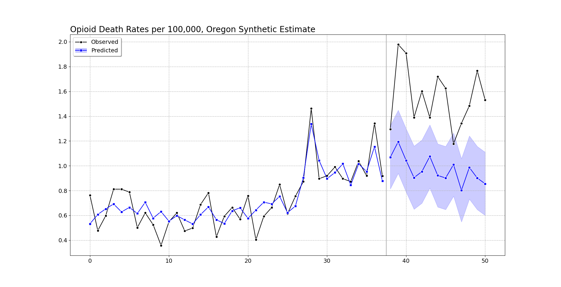
oregon.graph('Opioid Death Rates per 100,000, Oregon Synthetic Estimate')

So you can see the pre-intervention fit is smoother than the monthly data in Oregon, but by eye seems quite reasonable (matches the recent increase and spikes post period 20, starts in Jan-2018, so starting in August-2019). (Perfect fits are good evidence of over-fitting in machine learning.)

Post intervention, after period 37, I do my graph a bit differently. Sometimes people are confused when the intervention starts in the graph, so here I literally split pre/post data lines, so there should be no confusion. I use the conformal inference approach to generate 95% prediction intervals around the counterfactual trend. You can see the counterfactual trend has slightly decreased, whereas Oregon increased and is volatile. Some of the periods are covered by the upper most intervals, but the majority are clearly outside.

Now, besides the fitting function, one point I want to make is people should be looking at cumulative effects, not just instant effects. So Abadie has a global test, using placebos, that looks at the ratio of the pre-fit to post fit (squared errors), then does the placebo p-value based on that stat. This doesn’t have any consideration though for consistent above/below effects.

So pretend the Oregon observed was always within the 95% counterfactual error bar, but was always consistently at the top, around 0.1 increase in overdose deaths. Any single point-wise monthly inference fails to reject the null, but that overall always high pattern is not regular. You want to look at the entire curve, not just a single point. Random data won’t always be high or low, it should fluctuate around the counterfactual estimate.

To do this you look at the cumulative differences between the counterfactual and the observed (and take into account the error distribution for the counterfactuals).

# again default is 95% prediction intervals
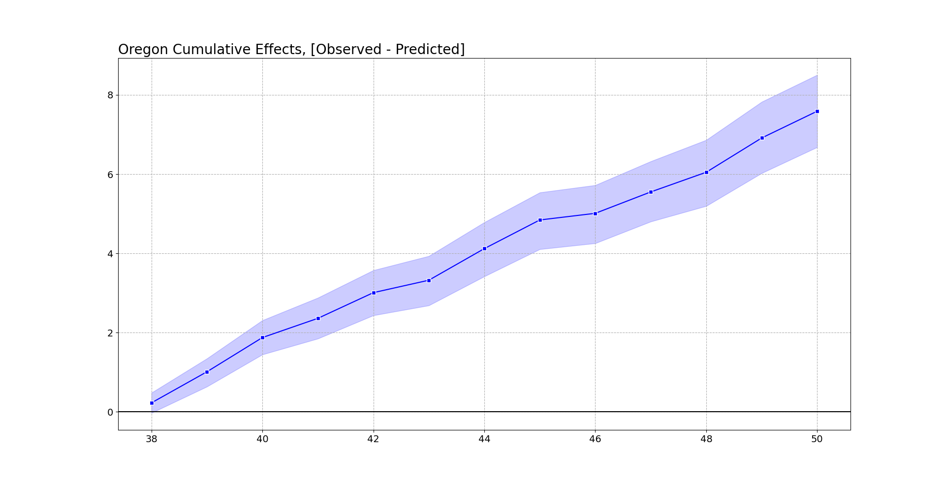
oregon.cumgraph('Oregon Cumulative Effects, [Observed - Predicted]')

Accumulated over time, this is a total of over 7 per 100,000. With Oregon having a population of around 4.1 million, I estimate that the cumulative increased number of overdose deaths is around 290 in Oregon. This is pretty consistent with the results in Spencer (2023) as well (182 increased deaths over fewer months).

To do a global test with this approach, you just look at the very final time period and whether it covers 0. This is what I suggest in-place of the Abadie permutation test, as this has a point estimate and standard error, not just a discrete p-value.

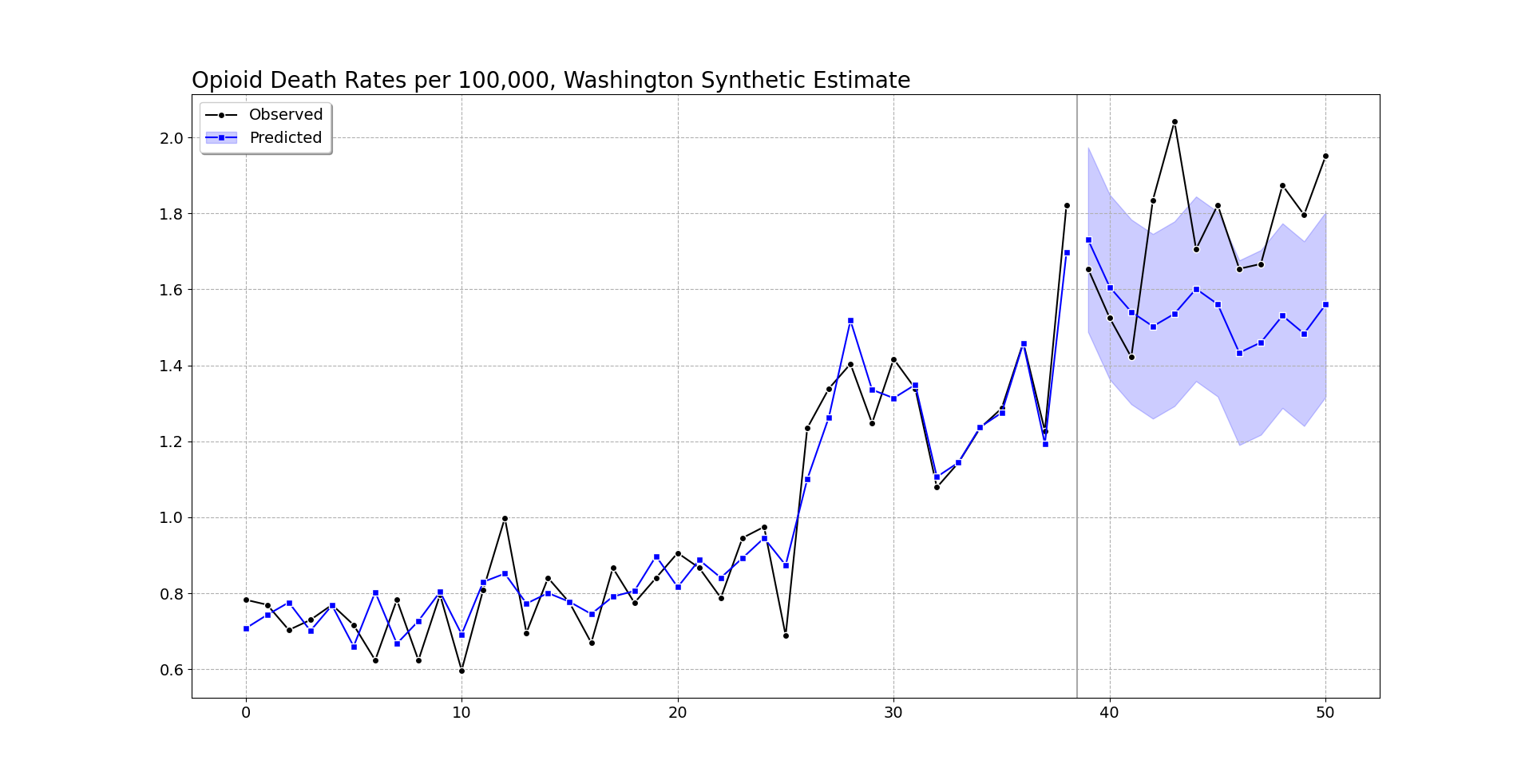
We can do the same analysis for Washington as we did for Oregon. It shows increases, but many of the time periods are covered by the counter-factual 95% prediction interval.

But like I mentioned before, they are consistently high. So when you do the cumulative effects for Washington, they more clearly show increases over time (this data last date is March 2022).

At an accumulated 2.5 per 100,000, with a state population of around 7.7 million, it is around 190 additional overdose deaths in Washington. You can check out the notebook for more stats, Washington has a smaller suggested alpha, so the matched weights have several more states. But the pre-fit is better, and so it has smaller counterfactual intervals. All again good things compared to the default (placebo approach Washington/Oregon will pretty much have the same error distribution, so Washington being less volatile does not matter using that technique).

I get that Abadie is an MIT professor, published a bunch in JASA and well known econ journals, and that his approach is standard in how people do synthetic control analyses. My experience though over time has made me think the default approaches here are not very good – and the placebo approach where you fit many alternative analyses just compounds the issue. (If the fit is bad, it makes the placebo results more variable, causing outlier placebos. People don’t go and do a deep dive of the 49 placebos though to make sure they are well behaved.)

The lasso + conformal approach is how I would approach the problem from my experience fitting machine learning models. I can’t give perfect proof this is a better technique than the SGD + placebo approach by Adadie, but I can release code to at least make it easier for folks to use this technique.

References

  • De Biasi, A., & Circo, G. (2021). Capturing crime at the micro-place: a spatial approach to inform buffer size. Journal of Quantitative Criminology, 37, 393-418.

  • Joshi, S., Rivera, B. D., Cerdá, M., Guy, G. P., Strahan, A., Wheelock, H., & Davis, C. S. (2023). One-year association of drug possession law change with fatal drug overdose in Oregon and Washington. JAMA Psychiatry Online First.

  • Piza, E. L., Wheeler, A. P., Connealy, N. T., & Feng, S. Q. (2020). Crime control effects of a police substation within a business improvement district: A quasi‐experimental synthetic control evaluation. Criminology & Public Policy, 19(2), 653-684.

  • Spencer, N. (2023). Does drug decriminalization increase unintentional drug overdose deaths?: Early evidence from Oregon Measure 110. Journal of Health Economics, 91, 102798.

Soft launching tech recruiting

I am soft-launching a tech recruiting service. I have had conversations with people on all sides of the equation on a regular basis, so I might as well make it a formal thing I do.

If you are an agency looking to fill a role, get in touch. If you are looking for a role, get in touch at https://crimede-coder.com/contact or send an email directly to andrew.wheeler@crimede-coder.com.

Why am I doing this?

I have a discussion with either a friend or second-degree friend about once a month who are current professors who ask me about making the jump to private sector. You can read my post, Make More Money, how I think many criminal justice professors are grossly underpaid. For PhD students you can see my advice at Flipping a CJ PhD to an Alt-Academic career.

If you are a current student or professor and want to chat, reach out and let me know you are interested. I am just going to start keeping a list of folks to help match them to current opportunities.

I have discussions with people who are trying to hire for jobs regularly as well. This includes police departments that are upping their game to hire more advanced roles, think tanks who want to hire early career individuals, and some tech companies in the CJ space who need to fill data science roles.

These are good jobs, and we have good people, so why are these agencies and businesses having a hard time filling these roles? Part of it is advertisement – these agencies don’t do a good job of getting the word out to the right audience. A second part is people have way off-base salary expectations (this is more common for academic positions, post docs I am looking at you). Part of the salary discussion is right sizing the role and expectations – you can’t ask for 10+ years experience and have a 90k salary for someone with an advanced degree – doesn’t really matter what job title you are hiring for.

I can help with both of those obviously – domain knowledge and my network can help your agency right size and fill that role.

Finally, I get cold messaged by recruiters multiple times a month. The straw to finally put this all on paper is I routinely encounter gross incompetence from recruiters. They do not understand the role the business is hiring for, they do not have expertise to evaluate potential candidates, and by cold emailing they clearly do not have a good network to pull potential candidates from.

If you are an agency or company whom you think my network of scholars can help fill your roll get in touch. I only get paid when you fill the position, so it is no cost to try to use my recruiting services. Again will help go over the role with you and say whether it feasible to fill that position as is, or whether it should be tweaked.

Below is my more detailed advice for job seekers. Again reach out if you are a job seeker, even if we have not met we can chat, I will see you do good work, and I will put you on my list of potential applicants to pull from in the future.

Tech Job Applying Advice, P1 Tech Roles

Here is an in-depth piece of advice I gave a friend recently – I think this will be useful in general to individuals in the social sciences who are interested in making the jump to the private sector.

First is understanding what jobs are available. This blog has a focus on quantitative work, but even if you do qualitative work there are tech opportunities. Also some jobs only need basic quant skills (Business Analyst) that any PhD will have (if you know how to use Excel and PowerPoint you have the necessary tech skills to be a business analyst).

Job labels and responsibilities are fuzzy, but here is a rundown of different tech roles and some descriptions:

  • Data Scientist
    • Role, fitting models and automating processes (writing code to shift data around)
    • need to have more advanced coding/machine learning background, e.g. have examples in python/R/SQL and know machine learning concepts
  • Business Analyst
    • anyone with a PhD can do this, Excel/Powerpoint
    • domain knowledge is helpful (which can be learned)
  • Program Manager/Project Manager
    • Help manage teams, roles are similar to “managing grants”, “supervising students”
    • often overlap with various project management strategies (agile, scrum).
    • These names are all stupid though, it is just supervising and doing “non-tech” things to help teams
  • Product Owner
    • Leads longer term development of a product, e.g. we should build X & Y in the next 3-6 months
    • Mix of tech or non-tech background (typically grow into this role from other prior roles)
    • If no tech need strong domain knowledge
    • Sometimes need to “sell” product, internally or externally
  • Director
    • Leads larger team of data scientists/programmers
    • Discusses with C-level, budgets/hiring/revenue projections
    • Often internal from Data Scientist or less often Product Owner/Business Analyst
    • but is possible to be direct into role with good domain knowledge

Salaries vary, it will generally be:

Business Analyst < Project Manager < {Data Scientist,Product Owner} < Director

But not always – tech highly values writing code, so it is not crazy for a supervisory role (Director) to make less than a senior Data Scientist.

Within Business Analyst you can have Junior/Senior (JR/SR) roles (for PhDs you should come in as Senior). Data scientist can have JR/SR/{Lead,Principal} (PhD should come in as Senior). JR needs supervision, SR can be by themselves and be OK, Lead is expected to mentor and supervise JRs.

Very generic salary ranges for typical cities (you should not take a job lower than the low end on these, with enough work you can find jobs higher, but will be hard in most markets):

  • Business Analyst: 70k – 120k
  • JR Data Scientist: 100k – 130k
  • SR Data Scientist: 130k – 180k
  • Program Manager: 100k – 150k
  • Product Owner: 120k – 160k
  • Director: 150k – 250k

Note I am not going to go and update this post (so this is September 2023), just follow up with me or do your own research to figure out typical salary ranges when this gets out of date in a year from now.

So now that you are somewhat familiar with roles, you need to find roles to apply to. There are two strategies; 1) find open roles online, 2) find specific companies. Big piece of advice here is YOU SHOULD BE APPLYING TO ROLES RIGHT NOW. Too many people think “I am not good enough”. YOU ARE GOOD ENOUGH TO APPLY TO 100s OF POSITIONS RIGHT NOW BASED ON YOUR PHD. Stop second guessing yourself and apply to jobs!

Tech Job Applying Advice, P2 Finding Positions

So one job strategy is to go to online job boards, such as LinkedIn, and apply for positions. For example, if I go search “Project Manager” in the Raleigh-Durham area, I get something like two dozen jobs pop-up. You may be (wrongly) thinking I don’t qualify for this job, buts lets look specifically at a job at NTT Data for a project manager, here are a few things they list:

  • Working collaboratively with product partners and chapter leaders to enable delivery of the squad’s mission through well-executed sprints
  • Accelerating overall squad performance, efficiency and value delivered by engaging within and across squads to find opportunities to improve agile maturity and metrics, and providing coaching, training and resources
  • Maintaining and updating squad performance metrics (e.g., burn-down charts) and artifacts to ensure accurate and clear feedback to the squad members and transparency to other partners
  • Managing, coordinating logistics for and participating in agile events (e.g., backlog prioritization, sprint planning, daily meetings, retrospectives and as appropriate, scrum of scrum masters)

This is all corporate gobbledygook for “managing a team to make sure people are doing their work on time” (and all the other bullet points are just more junk to say the same thing). You know who does that? Professors who supervise multiple students and manage grants.

For those with more quant programming skills, you have more potential opportunities (you can apply to data scientist jobs that require coding). But even if you do not have those skills, there are still plenty of opportunities.

Note that many of these jobs list “need to have” and “want to have”. You should still apply even if you do not meet all of the “need to have”. Very often these requirements will be made up and not actually “need to have” (it is common for job adverts to have obvious copy-paste mistakes or impossible need to haves). That NTT Data one has a “Certified Scrum Master (CSM) required” – if you see a bunch of jobs and that is what is getting you cut guess what? You can go and take a scrum master course in two days and check off that box. And have ChatGPT rewrite your cover letter asking it to sprinkle in agile buzzwords in the professor supervisory experience – people will never know that you just winged it when supervising students instead of using someone elses made up project management philosophy.

So I cannot say that your probability of landing any particular job is high, it may only be 1%. But unlike in academia, you can go on LinkedIn, and if you live in an urban area, likely find 100+ jobs that you could apply for right now (that pay more than a starting assistant professor in criminal justice).

So apply to many jobs, and most people I talk to with this strategy will be able to land something in 6-12 months. For resume/cover letter advice, here is my data science CV, and here is an example cover letter. For CV make it more focused on clear outcomes you have accomplished, instead of just papers say something like “won grant for 1 million dollars”, “supervised 5 students to Phd completion”, “did an RCT that reduced crime by 10%”. But you do not need to worry about making it only fit on 1 page (it can be multiple pages). Make it clear you have a PhD, people appreciate that, and people appreciate if you have a book published with a legit publisher as well (lay people find that more obviously impressive than peer reviewed publishing, because most people don’t know anything about peer reviewed publishing).

Do not bother tinkering to make different materials for every job (if the job requires cover letter, make generic and just swap out a few key words/company name). A cover letter will not make or break your job search, so don’t bother to customize it (I do not know how often they are even read).

Tech Job Applying Advice, P3 Finding Companies

The second strategy is to find companies you are interested in. Do you do work on drug abuse and victimization? There are probably healthcare companies you will be interested in. Do you do work tangentially related to fraud? Their are positions at banks who need machine learning skills. Are you interested in illegal markets? I bet various social media platforms need help with solutions to prevent selling illegal contraband.

This goes as well for think tanks (many cities have local think tanks that do good work, think beyond just RAND). These and civil service jobs (e.g. working for children and family services as an analyst) typically do not pay as high as private sector, but are still often substantially better than entry level assistant professor salaries (you can get think-tank or civil service gigs in the 80-120k range).

After you have found a company that you are interested in, you can go and look at open positions and apply to them (same as above). But an additional strategy at this point is to identify potential people you want to work with, and cold email/message them on social media.

It is similar to the above advice – many people will not answer your cold emails. It may be only 1/10 answer those emails. But an email is easy – there is no harm. Do not overthink it, send an email that is “Hey I think you do cool things, I do cool things too and would like to work together. Can we talk?” People will respond to something like that more often than you think. And if they don’t, it is their loss.

Here the biggest issue is a stigma associated with particular companies – people think Meta is some big evil company and they don’t want to work for them. And people think being an academic has some special significance/greater purpose.

If you go and build something for Meta that helps reduce illegal contraband selling by some miniscule fraction, you will have prevented a very large number of crimes. I build models that incrementally do a better job of identifying health care claims that are mis-billed. These models consistently generate millions of dollars of revenue for my company (and save several state Medicaid systems many millions more).

The world is a better place with me building stuff like that for the private sector. No doubt in my mind I have generated more value for society in the past 3 years than I would have in my entire career as an academic. These tech companies touch so many people, even small improvements can have big impacts.

Sorry to burst some academic bubbles, but that paper you are writing does not matter. It only matters to the extent you can get someone outside the ivory tower to alter their behavior in response to that paper. You can just cut out the academic middle man and work for companies that want to do that work of making the world a better place, instead of just writing about it. And make more money while you are it.

GUI Tool to download Google Streetview Imagery

For some brief updates, check out the newest post on the CRIME De-Coder blog, PDs should share crime data. I discuss the types of crime data PDs typically share, the benefit to doing so, and how it can be very easy (just upload a static file to a website).

Also wanted to share a new tool I built, a GUI interface to download multiple Google Streetview images given a list of addresses. Here is a video of the tool in action:

I have been asked in the past to do this based on several blog posts I have written (1,2). I get around 200 views of those posts per month, so figured it was worth some time to build something general to share – it is often people in marketing interested in that data.

I am selling the tool for $300. Check out the CRIME De-Coder Store to purchase. It is currently built for Windows, I can build it for Mac if there is demand. (If you have a list and just want me to download the images for you, e.g. you don’t want to sign up for a google API key yourself, just get in touch and I will give a quote based on your total volume.)

If you are wondering where the $300 pricing came in, there is a simple rule that if you can estimate the maximum price someone is willing to buy, divide by half and that is reasonably close to optimal on typical sloping downward demand curves. I had an offer for $600 for this recently, hence I set the price of the tool for $300.

If there is other web-scraping data you are interested, always feel free to get in touch. I can often give quick feedback as to the feasibility and give a quote for the work (as well as detail if what you are asking is even feasible given the data available).

Security issues with sending ChatGPT sensitive data

Part of my job as a data scientist is to be a bridge for lay-people interested in applying artificial intelligence and machine learning to their particular applications. Most quant people with a legit background will snicker at the term “artificial intelligence” – it is a buzzword for sure, but it doesn’t matter really. People have potential applications they need help with, and various statistical and optimization techniques can help.

Given the popularity of ChatGPT and other intelligent chatbots, I figured it would be worthwhile articulating the potential security issues with these technologies in criminal justice and healthcare domains. In particular, you should not send sensitive information in internet chatbot prompts. Examples of this include:

  • a crime analyst inputting incident narratives (that include names) and asking a chatbot to summarize them
  • a clinical coder inputting hospital notes and asking for the relevant billing codes
  • a business analyst inputting text from a set of slides, and asking ChatGPT to edit for grammer

The first two examples should be pretty clear why they are sensitive – they contain obviously sensitive and personal identifiable data. The last example is related to intellectual property leakage, which is more fuzzy, but for a general piece of advice if it is not OK to post publicly for everyone to see on the internet, you should not put it into a prompt. (So crime analysts talking about crime trends is probably OK, since that is already public info, but a business analyst with your pitch deck for internal business applications is probably not.)

Why can’t I send ChatGPT sensitive information?

So the way many online APIs work (including ChatGPT) is this:

  1. You go to website, you input information into a webform
  2. This data gets posted to a webpoint (someone elses computer)
  3. Someone elses computer takes that input, does something with that data
  4. That other computer sends information back to your computer

Here is a diagram of that flow:

So there are two potential attack vectors in this diagram. The first are the arrows sending data to/from OpenAIs computer. Someone could potentially intercept that data. This is not really a huge issue as stated, as the data is likely encrypted in transit. The second, and more important issue, is that the red OpenAI computer now has your sensitive data cached in some capacity.

If the red computer becomes compromised it can cause issues. This is not hypothetical, OpenAI has had issues of leaking sensitive information to other users. This is a computer glitch – bad but fixable. It is a risk though you should be aware of.

A more important issue though, the licensing I am aware of, they can use your conversations to improve the product. This is very bad as to my current understanding, as you can have conversations that are prompt leaked to third parties if they are updating models with your conversations downstream.

This is even worse than say Microsoft being able to read your emails – it would be like a potential third non-Microsoft party could become privy to some of your emails. For example, say a crime analyst in Raccoon city inputted crime incident narratives like I said in my prior example. Then I asked ChatGPT “Give me an example crime incident narrative”, and it outputs narratives very similar to the ones Raccoon city crime analyst previous put into ChatGPT. This is a feature under the current licensing, not a bug.

Let me know in the comments if they are offering paid tiers for the “don’t use my data for training and it is always encrypted and we can’t see it” (I don’t know why they do not offer that). Also they would need to have particular HIPPA standards for medical data, and CJIS standards for CJ data to be in security compliance for these example applications.

Now it is important to discuss other chatbots, who are often just calling OpenAI under the hood. The data flow diagram then looks like this:

It is essentially the same attack vectors but just doubled; now we have two computers instead of one that is a potential vulnerability.

Again here the issue is now two different people have your data cached in some capacity (the blue computer and the red computer). We have people making new services all the time now (the blue computers), that are just wrappers on OpenAI. Now you could have your data leaked by the blue computer, in addition to the problems with leaking in OpenAI.

The solution is local hosting, but local hosting is hard

OpenAI is to be commended for making a quality product – its very easy to use APIs are what make having wrapper services on top of it so easy (hence these many chatbot APIs). From a security standpoint though, you just need to do your due diligence now with two (or more) services when using these secondary tools, not just one. There will be malicious apps (so the blue computer is intentionally a bad actor), and there will be cases where the blue computer is compromised (so not intended to be malicious, but the people running the blue computer messed up).

Given that OpenAI as I am aware doesn’t have the necessary licensing to prevent info leakage, as well as the more specific security clearances, the solution like I said is to self host a model. Self hosting here means instead of sending data to the red OpenAI computer, the flow stays entirely in the single black computer you own, or you have your own server (so a second black computer that speaks to the first black computer).

There are open source and freemium models that are reasonable competitors. But, it is painful to self host these models. For neophytes the way these language models work, they take your text input, turn the text into a set of 1,000s of numbers. They then feed those 1,000s of numbers into a model with billions of parameters to get the final output. You can just think of it as doing several billion mathematical operations you individually could do on your hand-held calculator.

This takes a computer with a large memory and a GPU to do anything that doesn’t take hours. So self hosting a smaller batch process is maybe doable for a normal person or business, but if you want a live chatbot for even one person is hard (let alone a chatbot for multiple people to use at the same time).

Several large companies (including OpenAI) are currently even using up the majority of cloud infrastructure that has machines that can host and run these models, so even if you have money to pay AWS for one of their large GPU computers (it is expensive, think 5 digit costs per month), you maybe can’t even get a slot to get one of those cloud resources. And it is questionable how many people can even use that single machine.

I think eventually OpenAI will solve some of these security issues, and offer special paid tiers to accomodate use cases in healthcare and CJ. But until that happens, please do not post sensitive data into ChatGPT.

Age-Period-Cohort graphs for suicide and drug overdoses

When I still taught advanced research methods for PhD students, I debated on having a section on age-period-cohort (APC) analysis. Part of the reason I did not bother with that though is there were no good open source datasets (that I was aware of). A former student asking about APC analysis, as well as a recent NBER working paper on suicide rates (Marcotte & Hansen, 2023) brought it to mind again.

I initially had plans to do more modelling examples, but I decided on just showing off the graphs I generated. The graphs themselves I believe are quite informative.

So I went and downloaded mortality rates USA mortality rates for suicides and drug overdoses, spanning 1999-2022 for suicide and 1999-2021 for drug. Here is the data and R code to recreate these graphs in the post to follow along.

To follow along here in brief, we have a dataset of death and population counts, broken down by year and age:

# Age-Period-Cohort plots
library(ggplot2)

# Read in data
suicide <- read.csv('Suicides.csv')

# Calculate Rate & Cohort
suicide$Cohort <- suicide$Year - suicide$Age
suicide$Rate <- (suicide$Deaths/suicide$Population)*100000

# Suicide only 11-84
suicide <- suicide[suicide$Age >= 11,]
head(suicide)

And this produces the output:

> head(suicide)
   Age Year Deaths Population Cohort      Rate
16  11 1999     22    4036182   1988 0.5450696
17  11 2000     24    4115093   1989 0.5832189
18  11 2001     24    4344913   1990 0.5523701
19  11 2002     22    4295720   1991 0.5121377
20  11 2003     15    4254047   1992 0.3526054
21  11 2004     18    4207721   1993 0.4277850

A few notes here. 1) I limited the CDC Vital stats data to 1999, because in the Wonder dataset pre-1999 you can’t get individual year-age breakdowns, you need to do 5 year age bins. This can cause issues where you need to age-adjust within those bins (Gelman & Auerbach, 2016), that should be less of a problem with single year breakdowns. So I would go back further were it not for that. 2) When breaking down to individual years, the total count of suicides per age bracket is quite small. Initially I was skeptical of Marcotte & Hansen’s (2023) claims of LGBTQ subgroups potentially accounting for increased trends among young people (I just thought that group was too small for that to make sense), but looking at the counts I don’t think that is the case.

When I think about age-period-cohort analysis, my mind goes age effects > period effects > cohort effects. I think people often mix up cohort effects with things that are actually age effects. (And also generation labels are not real.) In criminology, the age-crime-curve was established back in the 1800’s by Quetelet.

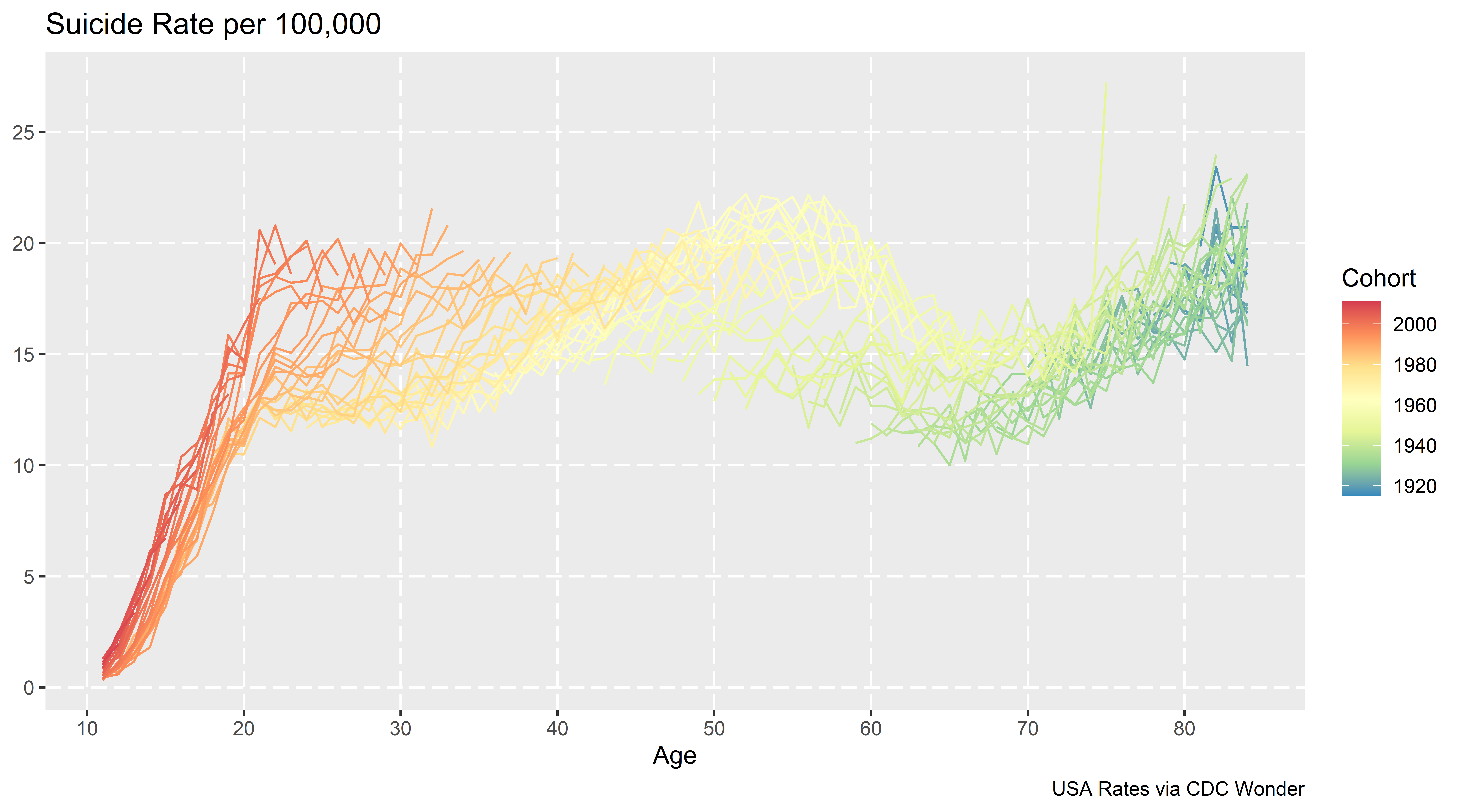
So I focus on graphing the age curve, and look at deviations from that to try to visually identify period effects or cohort effects. Here is the plot to look at each of the age curves, broken down by year.

ap <- ggplot(data=suicide, aes(x = Age, y = Rate, color=Year, group=Year)) + 
             geom_line() +
             scale_colour_distiller(palette = "PuOr") +
             scale_x_continuous(breaks=seq(10,80,10)) +
             scale_y_continuous(breaks=seq(0,30,5)) + 
             labs(x='Age',y=NULL,title='Suicide Rate per 100,000',caption="USA Rates via CDC Wonder")
ap

When using diverging color ramps to visualize a continuous variable, you get a washed out effect in the middle. So I am not sure the best color ramp here, but it does provide a nice delineation and gradual progression from the curve in the early 2000’s compared to the suicide curve in 2022. (Also spot the one outlier year, it is age 75 for the “provisional” 2022 counts. I leave it in as it is a good showcase for how plots can help spot bad data.)

The blog the graph will be tinier, open it up in a new tab on your desktop computer to get a good look at the full size image.

Here looking at the graph you can see two things other researchers looking at similar data have discussed. In the early 2000’s, you had a gradual increase from 20’s to the peak suicide rate at mid 40’s. More recent data has shifted that peak to later ages, more like peak 55. Case & Deaton (2015) discussing deaths of despair (of which suicide is a part) focussed on this shift, and noted that females in this age category increased at a higher rate relative to males.

Marcotte & Hansen (2023) focus on the younger ages. So in the year 2000, the age-suicide curve was a gradual incline from ages early 20’s until the peak. Newer cohorts though show steeper inclines in the earlier ages, so the trend from ages 20-60 is flatter than before.

Period effects in these charts will look like the entire curve is the same shape, and it is just shifted up and down. (It may be better to graph these as log rates, but keeping on the linear scale for simplicity.) We have a bit of a shape change though, so these don’t rule out cohort effects.

Here is the same plot, but grouping by cohorts instead of years. So the age-suicide curve is indexed to the birth year for an individual:

cp <- ggplot(data=suicide, aes(x = Age, y = Rate, color=Cohort, group=Cohort)) + 
             geom_line() +
             scale_colour_distiller(palette = "Spectral") +
             scale_x_continuous(breaks=seq(10,80,10)) +
             scale_y_continuous(breaks=seq(0,30,5)) +
             labs(x='Age',y=NULL,title='Suicide Rate per 100,000',caption="USA Rates via CDC Wonder")
cp

My initial cheeky thought (not that there aren’t enough ways to do APC models already), was to use mixture models to identify discrete cohorts. Something along the lines of this in the R flexmix package (note this does not converge):

library(flexmix)
knot_loc <- c(20,35,50,65) # for ages
model <- stepFlexmix(cbind(Deaths, Population - Deaths) ~ bs(Age, knot_loc) | Cohort, 
                     model = FLXMRglm(family = "binomial", fixed = ~Year),
                     data = suicide, k = 3)

But there is an issue with this when looking at the cohort plot, you have missing data for cohorts – to do this you would need to observe the entire age-curve for a cohort. There may be a way to estimate this using latent class models in Stata (and fixing some of the unidentified spline coefficients to a fixed value), but to me just looking at the graphs I think is all I really care about. You could maybe say the orange cohorts in the late 90’s are splitting off, but I think that is consistent with period effects. (And is also a trick of the colors I used in the plot.)

You could do mixtures for the year plots, see some of the work by Elana Erosheva (Erosheva et al., 2014), but that again just isn’t how I think about APC analysis.

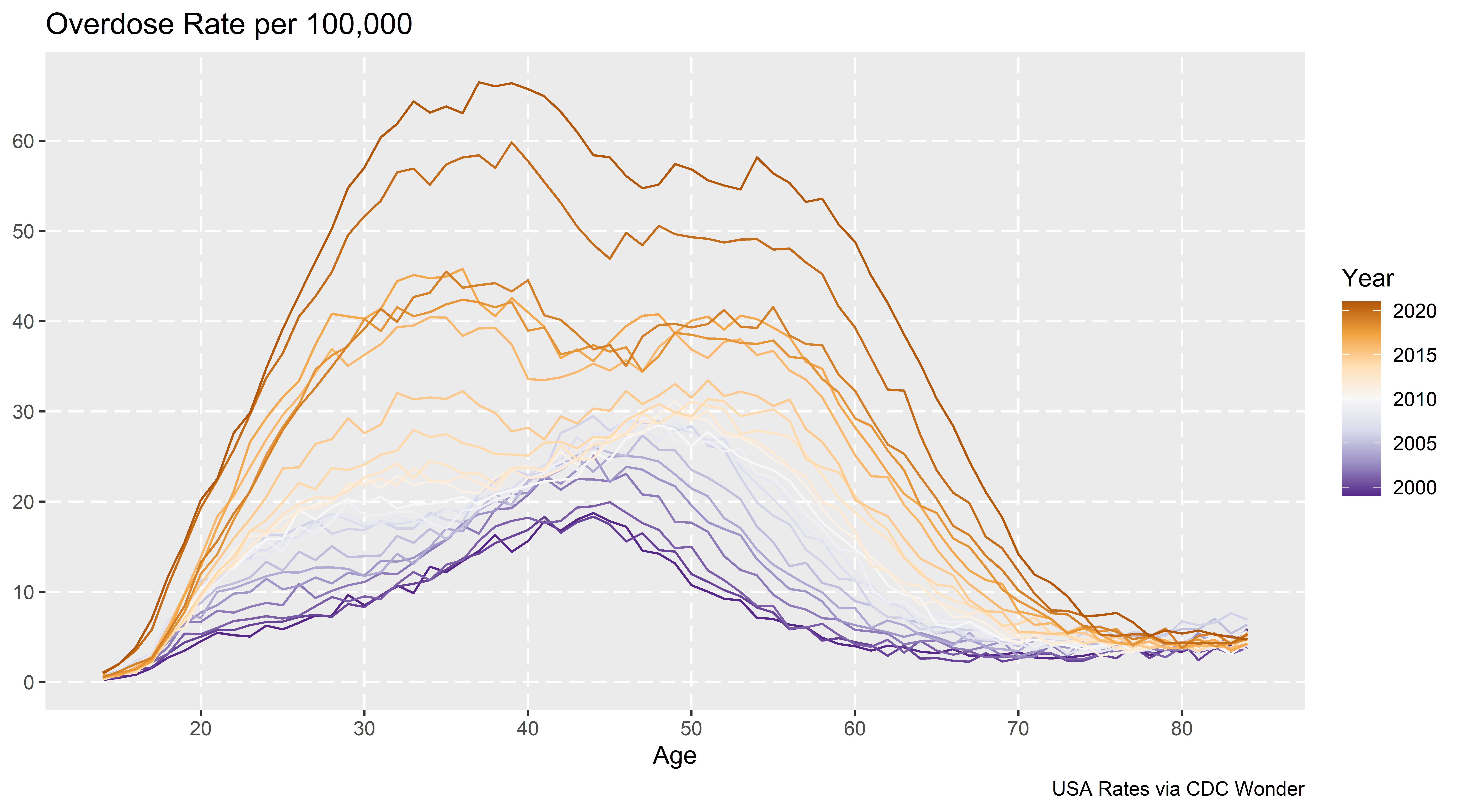
Doing this same exercise for drug overdoses rates, (which I not can overlap with suicide – you can commit suicide via intentionlly taking too many drugs) we can clearly see the dramatic rise in recent years. We can also see the same trends in earlier ages now being peak, but also increases and shifts to older ages.

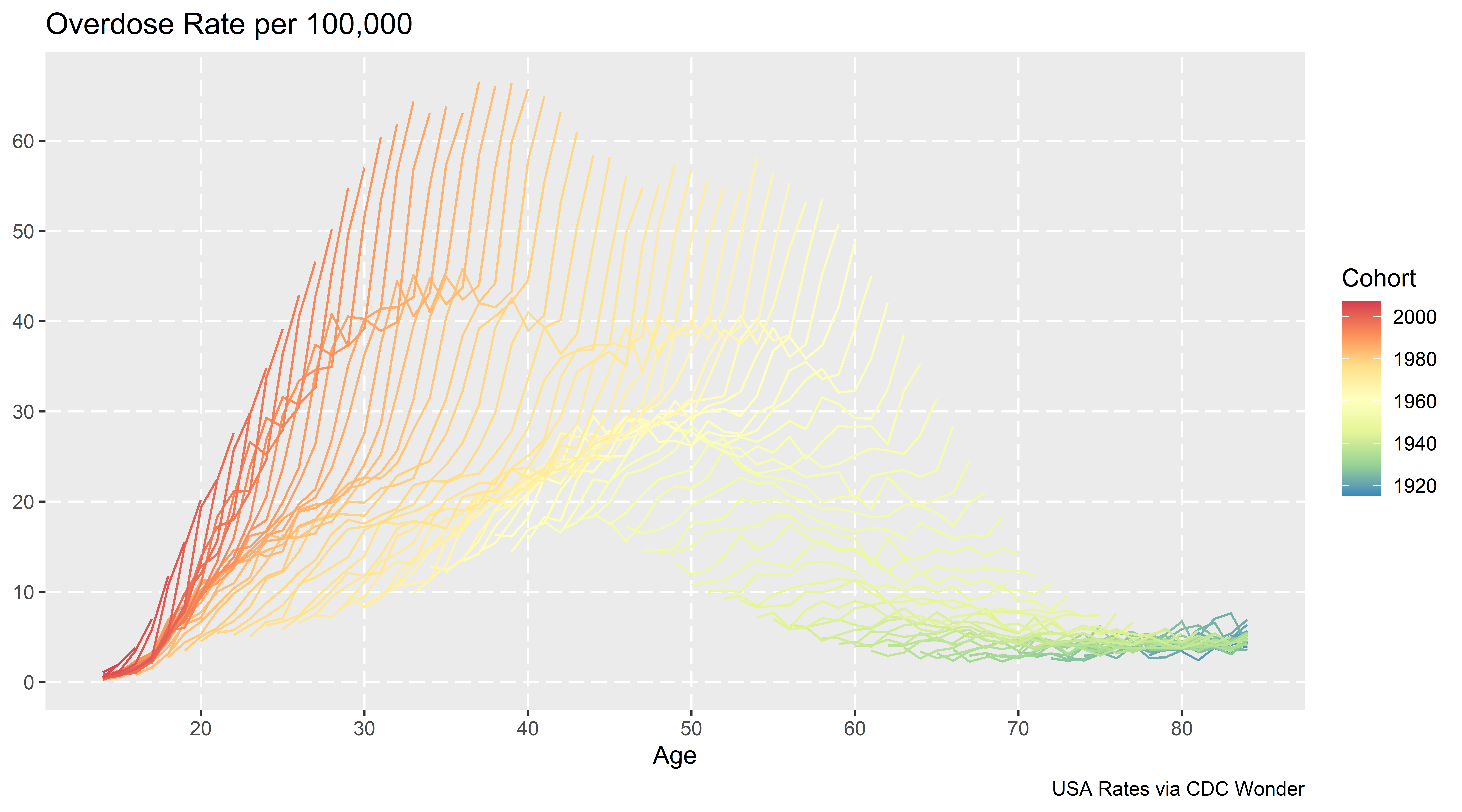
The cohort plot here looks like a Spinosaurus crest:

Which I believe is more consistent with (very strong) period effects, not so much cohort effects. Drug overdoses are increasing across both younger and older cohorts.

Nerd Notes

These datasets don’t have covariates, which to use the APC method in Spelman (2022) you would need those (it uses covariates to estimate period effects). I am not so sure that is the best approach to APC decomposition, but it is horses for courses.

What I wish is that the CDC distributed the vital statistics data at the micro level (where each row is a death, with all of the covariates), along with a matching variable dataset of the micro level American Community Survey and the weights. That doesn’t solve the APC issue with identifying the different effects, but makes it easier to do more complicated modelling, e.g. I could fit models or generate graphs for age-gender differences more easily, decompose different death types, etc.

Final nerd note is about forecasting mortality trends. While I am familiar with the PCA-functional data approach advocated by Rob Hyndman (Hyndman & Ullah, 2007), I don’t think that will do very well with this data. I am wondering if doing some type of multi-level GAM model, and doing short term extrapolation of the period effect (check out Gavin Simpson’s posts on multi-level smooths, 1, 2, 3).

So maybe something like:

library(mgcv)
smooth_model <- gam(cbind(Deaths, Population - Deaths) ~ s(Year) + s(Age,by=Cohort), 
                    family = binomial("logit"),
                    data = suicide)

Or maybe just use s(Age,Year) and not worry about the cohort effect. Caveat emptor about this model, this is just my musings, I have not in-depth studied it to make sure it behaves well (although a quick check R does not complain when fitting it).

References

Too relaxed? Naive Bayes does not improve recidivism forecasting in the NIJ challenge

So the paper Improving Recidivism Forecasting With a Relaxed Naïve Bayes Classifier (Lee et al., 2023), recently published in Crime & Delinquency, has incorrect results. Note I am not sandbagging on the authors, I reviewed this paper for JQC and Journal of Criminal Justice, so I have given the authors this same feedback already (multiple times!). The authors however did not correct their results, and just journal shopped and published the wrong findings.

I have replication code here to review. (Note I initially made a mistake in my code replication, reversed calculating p(x|y), I calculated p(y|x) by accident, see this older code I shared in my prior reviews, but I was still correct in my assertion that Lee’s results were wrong.)

So the main thing that made me go to this effort, the authors report unbelieveable results. They report Brier Scores for Females (Round 1) of 0.104 and for males 0.159 – these scores blow the competition out of the water. The leaderboard was 0.15 for Females and 0.19 for males. Note how I don’t list to the third decimal – the difference between the teams you needed to go down that low. Lee also reports unbelievably low Brier scores for the alternative logit and random forest models – their results just on their face are not believable.

If the authors really believe their results this kind of sucks for them they did not participate in the NIJ challenge, they would have won more than $150,000! But I am pretty sure they are miscalculating their Brier scores somewhere. My replication code shows them in the same ballpark as everyone else, but they would not have made the leaderboard. Here are my estimates of what their Brier scores should be reported as (the Brier column below in the two tables):

Folks can go and look at their paper and their set of spreadsheets in the supplemental material – I have posted not many more than 50 lines of (non-comment) python code that replicates their regression model coefficients and shows their Brier scores are wrong though. (And subsequently any points Lee et al. 2023 make about fairness are thus wrong as well.)

NIJ probably released papers at some point, but if you want to see other folks discussion, there is Circo & Wheeler (2022) (for mine and Gio’s results for team MCHawks), and Mohler & Porter (2021) for team PASDA.

I may put in the slate sometime to discuss naive Bayes (and other categorical encoding schemes). It is not a bad idea for data with many categories, but for this NIJ data there just isn’t that much to squeeze out of the data. So any future work will be unlikely to dramatically improve upon the competition results (it is difficult to overfit this data). Again given my analysis here, I am pretty sure a valid data analysis (not peeking) at best will “beat” the competition results in the 3rd decimal place (if they can improve at all).

Now part of the authors argument is that this method (relaxed naive Bayes) results in simpler interpretations. Typically people interpret “simple” models in terms of the end results, e.g. having a simple checklist of integer weights. The more I deal with predictive models though, I think this is maybe misguided. You could also interpret “simple” in terms of the code used for how someone derived the weights (and evaluated the final metrics). This is important when auditing code that others have written, as you will ultimately take the code and apply it to your data.

I think this “simpler to estimate the same results” is probably more important for scientists and outside groups wanting to verify the integrity of any particular machine learning model than “simple end result weights”. Otherwise scientists can make up results and say my method is better. Which is simpler I suppose, but misses the boat a bit in terms of why we want simple models to begin with.

References

Some notes on synthetic control and Hogan/Kaplan

This will be a long one, but I have some notes on synthetic control and the back-and-forth between two groups. So first if you aren’t familiar, Tom Hogan published an article on how the progressive District Attorney (DA) in Philadelphia, Larry Krasner, in which Hogan estimates that Krasner’s time in office contributed to a large increase in the number of homicides. The control homicides are estimated using a statistical technique called synthetic control, in which you derive estimates of the trend in homicides to compare Philly to based on a weighted average of comparison cities.

Kaplan and colleagues (KNS from here on) then published a critique of various methods Hogan used to come up with his estimate. KNS provided estimates using different data and a different method to derive the weights, showing that Philadelphia did not have increased homicides post Krasner being elected. For reference:

Part of the reason I am writing this is if people care enough, you could probably make similar back and forths on every synth paper. There are many researcher degrees of freedom in the process, and in turn you can make reasonable choices that lead to different results.

I think it is worthwhile digging into those in more detail though. For a summary of the method notes I discuss for this particular back and forth:

  • Researchers determine the treatment estimate they want (counts vs rates) – solvers misbehaving is not a reason to change your treatment effect of interest
  • The default synth estimator when matching on counts and pop can have some likely unintended side-effects (NYC pretty much has to be one of the donor cities in this dataset)
  • Covariate balancing is probably a red-herring (so the data issues Hogan critiques in response to KNS are mostly immaterial)

In my original draft I had a note that this post would not be in favor of Hogan nor KNS, but in reviewing the sources more closely, nothing I say here conflicts with KNS (and I will bring a few more critiques of Hogan’s estimates that KNS do not mention). So I can’t argue much with KNS’s headline that Hogan’s estimates are fatally flawed.

An overview of synthetic control estimates

To back up and give an overview of what synth is for general readers, imagine we have a hypothetical city A with homicide counts 10 15 30, where the 30 is after a new DA has been elected. Is the 30 more homicides than you would have expected absent that new DA? To answer this, we need to estimate a counterfactual trend – what the homicide count would have been in a hypothetical world in which a new progressive DA was not elected. You can see the city homicides increased the prior two years, from 10 to 15, so you may say “ok, I expected it to continue to increase at the same linear trend”, in which case you would have expected it to increase to 20. So the counterfactual estimated increase in that scenario is observed - counterfactual, here 30 - 20 = 10, an estimated increase of 10 homicides that can be causally attributed to the progressive DA.

Social scientists tend to not prefer to just extrapolate prior trends from the same location into the future. There could be widespread changes that occur everywhere that caused the increase in city A. If homicide rates accelerated in every city in the country, even those without a new progressive DA, it is likely something else is causing those increases. So say we compare city A to city B, and city B had a homicide count trend during the same time period 10 15 35. Before the new DA in city A, cities A/B had the same pre-trend (both 10 15). The post time period City B increased to 35 homicides. So if using City B as the counterfactual estimate, we have the progressive DA reduced 5 homicides, again observed - counterfactual = 30 - 35 = -5. So even though city A increased, it increased less than we expected based on the comparison city B.

Note that this is not a hypothetical concern, it is pretty basic one that you should always be concerned about when examining macro level crime data. There has been national level homicide increases over the time period when Krasner has been in office (Yim et al, 2020, and see this blog post for updates. U.S. city homicide rates tend to be very correlated with each other (McDowall & Loftin, 2009).

So even though Philly has increased in homicide counts/rates when Krasner has been in office, the question is are those increases higher or lower than we would expect. That is where the synthetic control method comes in, we don’t have a perfect city B to compare to Philadelphia, so we create our own “synthetic” counter-factual, based on a weighted average of many different comparison cities.

To make the example simple, imagine we have two potential control cities and homicide trends, city C1 0 30 20, and city C2 20 0 30. Neither looks like a good comparison to city A that has trends 10 15 30. But if we do a weighted average of C1 and C2, with the weights 0.5 for each city, when combined they are a perfect match for the two pre-treatment periods:

C0  C1 Average cityA
 0  20   10     10
30   0   15     15
20  30   25     30

This is what the synthetic control estimator does, although instead of giving equal weights it determines the optimal weights to match the pre-treatment time period given many potential donors. In real data for example C0 and C1 may be given weights of 0.2 and 0.8 to give the correct balance based on the prior to treatment time periods.

The fundamental problem with synth

The rub with estimating the synth weights is that there is no one correct way to estimate the weights – you have more numbers to estimate than data points. In the Hogan paper, he has 5 pre time periods, 2010-2014, and he has 82 potential donors (99 other of the largest cities in the US minus 17 progressive prosecutors). So you need to learn 82 numbers (the weights) based on 5 data points.


Side note: you can also consider matching on covariates additional data points, although I will go into more detail on how matching on covariates is potentially a red-herring. Hogan I think uses an additional 5*3=15 time varying points (pop, cleared homicide, homicide clearance rates), and maybe 3 additional time invariant (median income, 1 prosecutor categorization, and homicides again!). So maybe has 5 + 15 + 3 = 23 data points to match on (so same fundamental problem, 23 numbers to learn 82 weights). I am just going to quote the full passage on Hogan (2022a) here where he discusses covariate matching:

The number of homicides per year is the dependent variable. The challenge with this synthetic control model is to use variables that both produce parallel trends in the pre-period and are sufficiently robust to power the post-period results. The model that ultimately delivered the best fit for the data has population, cleared homicide cases, and homicide clearance rates as regular predictors. Median household income is passed in as the first special predictor. The categorization of the prosecutors and the number of homicides are used as additional special predictors. For homicides, the raw values are passed into the model. Abadie (2021) notes that the underlying permutation distribution is designed to work with raw data; using log values, rates, or other scaling techniques may invalidate results.

This is the reason why replication code is necessary – it is very difficult for me to translate this to what Hogan actually did. “Special” predictors here are code words for the R synth package for time-invariant predictors. (I don’t know based on verbal descriptions how Hogan used time-invariant for the prosecutor categorization for example, just treats it as a dummy variable?) Also only using median income – was this the only covariate, or did he do a bunch of models and choose the one with the “best” fit (it seems maybe he did do a search, but doesn’t describe the search, only the end selected result).

I don’t know what Hogan did or did not do to fit his models. The solution isn’t to have people like me and KNS guess or have Hogan just do a better job verbally describing what he did, it is to release the code so it is transparent for everyone to see what he did.


So how do we estimate those 82 weights? Well, we typically have restrictions on the potential weights – such as the weights need to be positive numbers, and the weights should sum to 1. These are for a mix of technical and theoretical reasons (having the weights not be too large can reduce the variance of the estimator is a technical reason, we don’t want negative weights as we don’t think there are bizzaro comparison areas that have opposite world trends is a theoretical one).

These are reasonable but ultimately arbitrary – there are many different ways to accomplish this weight estimation. Hogan (2022a) uses the R synth package, KNS use a newer method also advocated by Abadie & L’Hour (2021) (very similar, but tries to match to the closest single city, instead of weights for multiple cities). Abadie (2021) lists probably over a dozen different procedures researchers have suggested over the past decade to estimate the synth weights.

The reason I bring this up is because when you have a problem with 82 parameters and 5 data points, the problem isn’t “what estimator provides good fit to in-sample data” – you should be able to figure out a estimator that accomplishes good in-sample fit. The issue is whether that estimator is any good out-of-sample.

Rates vs Counts

So besides the estimator used, you can break down 3 different arbitrary researcher data decisions that likely impact the final inferences:

  • outcome variable (homicide counts vs homicide per capita rates)
  • pre-intervention time periods (Hogan uses 2010-2014, KNS go back to 2000)
  • covariates used to match on

Lets start with the outcome variable question, counts vs rates. So first, as quoted above, Hogan cites Abadie (2021) for saying you should prefer counts to rates, “Abadie (2021) notes that the underlying permutation distribution is designed to work with raw data; using log values, rates, or other scaling techniques may invalidate results.”

This has it backwards though – the researcher chooses whether it makes sense to estimate treatment effects on the count scale vs rates. You don’t goal switch your outcome because you think the computer can’t give you a good estimate for one outcome. So imagine I show you a single city over time:

        Y0    Y1    Y2
Count   10    15    20
Pop   1000  1500  2000

You can see although the counts are increasing, the rate is consistent over the time period. There are times I think counts make more sense than rates (such as cost-benefit analysis), but probably in this scenario the researcher would want to look at rates (as the shifting denominator is a simple explanation causing the increase in the counts).

Hogan (2022b) is correct in saying that the population is not shifting over time in Philly very much, but this isn’t a reason to prefer counts. It suggests the estimator should not make a difference when using counts vs rates, which just points to the problematic findings in KNS (that making different decisions results in different inferences).

Now onto the point that Abadie (2021) says using rates is wrong for the permutation distribution – I don’t understand what Hogan is talking about here. You can read Abadie (2021) for yourself if you want. I don’t see anything about the permutation inferences and rates.

So maybe Hogan mis-cited and meant another Abadie paper – Abadie himself uses rates for various projects (he uses per-capita rates in the 2021 cited paper, Abadie et al., (2010) uses rates for another example), so I don’t think Abadie thinks rates are intrinsically problematic! Let me know if there is some other paper I am unaware of. I honestly can’t steelman any reasonable source where Hogan (2022a) came up with the idea that counts are good and rates are bad though.

Again, even if they were, it is not a reason to prefer counts vs rates, you would change your estimator to give you the treatment effect estimate you wanted.


Side note: Where I thought the idea with the problem with rates was going (before digging in and not finding any Abadie work actually saying there is issues with rates), was increased variance estimates with homicide data. So Hogan (2022a) estimates for the synth weights Detroit (0.468), New Orleans (NO) (0.334), and New York City (NYC) (0.198), here are those cities homicide rates graphed (spreadsheet with data + notes on sources).

You can see NO’s rate is very volatile, so is not a great choice for a matched estimator if using rates. (I have NO as an example in Wheeler & Kovandzic (2018), that much variance though is fairly normal for high crime not too large cities in the US, see Baltimore for example for even more volatility.) I could forsee someone wanting to make a weighted synth estimator for rates, either make the estimator a population weighted average, or penalize the variance for small rates. Maybe you can trick microsynth to do a pop weighted average out of the box (Robbins et al., 2017).


To discuss the Hogan results specifically, I suspect for example NYC being a control city with high weight in the Hogan paper, which superficially may seem good (both large cities on the east coast), actually isn’t a very good control area considering the differences in homicide trends (either rates or counts) over time. (I am also not so sure about describing NYC and New Orlean’s as “post-industrial” by Hogan (2022a) either. I mean this is true to the extent that all urban areas in the US are basically post-industrial, but they are not rust belt cities like Detroit.)

Here is for reference counts of homicides in Philly, Detroit, New Orleans, and NYC going back further in time:

NYC is such a crazy drop in the 90s, lets use the post 2000 data that KNS used to zoom in on the graph.

I think KNS are reasonable here to use 2000 as a cut point – it is more empirical based (post crime drop), in which you could argue the 90’s are a “structural break”, and that homicides settled down in most cities around 2000 (but still typically had a gradual decline). Given the strong national homicide trends though across cities (here is an example I use for class, superimposing Dallas/NYC/Chicago), I think using even back to the 60’s is easily defensible (moreso than limiting to post 2010).

It depends on how strict you want to be whether you consider these 3 cities “good” matches for the counts post 2010 in Hogan’s data. Detroit seems a good match on the levels and ok match on trends. NO is ok match on trends. NYC and NO balance each other in terms of matching levels, NYC has steeper declines though (even during the 2010-2014 period).

The last graph though shows where the estimated increases from Hogan (2022a) come from. Philly went up and those 3 other cities went down from 2015-2018 (and had small upward bumps in 2019).

Final point in this section, careful what you wish for with sparse weights and sum to 1 in the synth estimate. What this means in practice when using counts and matching on pop size, is that you need lines that are above and below Philly on those dimensions. So to get a good match on Pop, it needs to select at least one of NYC/LA/Houston (Chicago was eliminated due to having a progressive prosecutor). To get a good match on homicide counts, it also has to pick at least one city with more homicides per year as well, which limits the options to New York and Detroit (LA/Houston have lower overall homicide counts to Philly).

You can’t do the default Abadie approach for NYC for example (matching on counts and pop) – it will always have a bad fit when using comparison cities in the US as the donor pool. You either need to allow the weights to sum to larger than 1, or the lasso approach with an intercept is another option (so you only match on trend, not levels).

Because matching on trends is what matters for proper identification in this design, not levels, this is all sorts of problematic with the data at hand. (This is also a potential problem with the KNS estimator as well. KNS note though they don’t trust their estimate offhand, their reasonable point is that small changes in the design result in totally different inferences.)

Covariates and Out of Sample Estimates

For sake of argument, say I said Hogan (2022a) is bunk, because it did not match on “per-capita annual number of cheese-steaks consumed”. Even though on its face this covariate is non-sense, how do you know it is non-sense? In the synthetic control approach, there is no empirical, falsifiable way to know whether an covariate is a correct one to match on. There is no way to know that median income is better than cheese-steaks.

If you wish for more relevant examples, Philly has obviously more issues with street consumption of opioids than Detroit/NOLA/NYC, which others have shown relationships to homicide and has been getting worse over the time Krasner has been in office (Rosenfeld et al., 2023). (Or more simply social disorganization is the more common way that criminologists think about demographic trends and crime.)

This uncertainty in “what demographics to control for” is ok though, because matching on covariates is neither necessary nor sufficient to ensure you have estimated a good counter-factual trend. Abadie in his writings intended for covariates to be more like fuzzy guide-rails – they are qualitative things that you think the comparison areas should be similar on.

Because there are effectively an infinite pool of potential covariates to match on, I prefer the approach of simply limiting the donor pool apriori – Hogan limiting to large cities is on its face reasonable. Including other covariates is not necessary, and does not make the synth estimate more or less robust. Whether KNS used good or bad data for covariates is entirely a red-herring as to the quality of the final synth estimate.


Side note: I don’t doubt that Hogan got advice to not share data and code. It is certainly not normative in criminology to do this. It creates a bizarre situation though, in which someone can try to replicate Hogan by collating original sources, and then Hogan always comes back and says “no, the data you have are wrong” or “the approach you did is not exactly replicating my work”.

I get that collating data takes a long time, and people want to protect their ability to publish in the future. (Or maybe just limit their exposure to their work being criticized.) It is blatantly antithetical to verifying the scientific integrity of peoples work though.

Even if Hogan is correct though in the covariates that KNS used are wrong, it is mostly immaterial to the quality of the synth estimates. It is a waste of time for outside researchers to even bother to replicate Hogan’s covariates he used.


So I used the idea of empirical/falsifiable – can anything associated with synth be falsifiable? Why yes it can – the typical approach is to do some type of leave-one-out estimate. It may seem odd because synth estimates an underlying match to a temporal trend in the treated location, but there is nothing temporal about the synth estimate. You could jumble up the years in the pre-treatment sample and still would estimate the same weights.

Because of this, you can leave-a-year-out in the pre-treatment time period, run your synth algorithm, and then predict that left out year. A good synth estimator will be close to the observed value for the out of sample estimates in the pre-treated time period (and as a side bonus, you can use that variance estimate to estimate the error in the post-trend years).

That is a relatively simple way to determine if the Hogan 5 year vs KNS 15 year time periods are “better” synth controls (my money is on KNS for that one). Because Hogan has not released data/code, I am not going to go through that trouble. As I said in the side note earlier, I could try to do that, and Hogan could simply come back and say “you didn’t do it right”.

This also would settle the issue of “over-fit”. You actually cannot just look at the synth weights, and say that if they are sparse they are not over-fit and if not sparse are over-fit. So for reference, you have in Hogan essentially fitting 82 weights based on 5 datapoints, and he identified a fit with 3 non-zero weights. Flip this around, and say I had 5 data points and fit a model with 3 parameters, it is easily possible that the 3 parameter model in that scenario is overfit.

Simultaneously, it is not necessary to have a sparse weights matrix. Several alternative methods to estimate synth will not have sparse weights (I am pretty sure Xu (2017) will not have sparse weights, and microsynth estimates are not sparse either for just two examples). Because US cities have such clear national level trends, a good estimator in this scenario may have many tiny weights (where good here is low bias and variance out of sample). Abadie thinks sparse weights are good to make the model more interpretable (and prevent poor extrapolation), but that doesn’t mean by default a not sparse solution is bad.

To be clear, KNS admit that their alternative results are maybe not trustworthy due to not sparse weights, but this doesn’t imply Hogan’s original estimates are themselves “OK”. I think maybe a correct approach with city level homicide rate data will have non-sparse weights, due to the national level homicide trend that is common across many cities.

Wrapping Up

If Crim and Public Policy still did response pieces maybe I would go through that trouble of doing the cross validation and making a different estimator (although I would unlikely be an invited commenter). But wanted to at least do this write up, as like I said at the start I think you could do this type of critique with the majority of synth papers in criminology being published at the moment.

To just give my generic (hopefully practical) advice to future crim work:

  • don’t worry about matching on covariates, worry about having a long pre-period
  • the default methods you need to worry about if you have enough “comparable” units – this is in terms of levels, not just trends
  • the only way to know the quality of the modeling procedure in synth is to do out of sample estimates.

Bullet points 2/3 are perhaps not practical – most criminologists won’t have the capability to modify the optimization procedure to the situation at hand (I spent a few days trying without much luck to do my penalized variants suggested, sharing so others can try out themselves, I need to move onto other projects!) Also takes a bit of custom coding to do the out of sample estimates.

For many realistic situations though, I think criminologists need to go beyond just point and clicking in software, especially for this overdetermined system of equations synthetic control scenario. I did a prior blog post on how I think many state level synth designs are effectively underpowered (and suggested using lasso estimates with conformal intervals). I think that is a better default in this scenario as well compared to the typical synth estimators, although you have plenty of choices.

Again I had initially written this as trying to two side the argument, and not being for or against either set of researchers. But sitting down and really reading all the sources and arguments, KNS are correct in their critique. Hogan is essentially hiding behind not releasing data and code, and in that scenario can make an endless set of (ultimately trivial) responses of anyone who publishes a replication/critique.

Even if some of the the numbers KNS collated are wrong, it does not make Hogan’s estimates right.

References

Youtube interview with Manny San Pedro on Crime Analysis and Data Science

I recently did an interview with Manny San Pedro on his YouTube channel, All About Analysis. We discuss various data science projects I conducted while either working as an analyst, or in a researcher/collaborator capacity with different police departments:

Here is an annotated breakdown of the discussion, as well as links to various resources I discuss in the interview. This is not a replacement for listening to the video, but is an easier set of notes to link to more material on what particular item I am discussing.

0:00 – 1:40, Intro

For rundown of my career, went to do PhD in Albany (08-15). During that time period I worked as a crime analyst at Troy, NY, as well as a research analyst for my advisor (Rob Worden) at the Finn Institute. My research focused on quant projects with police departments (predictive modeling and operations research). In 2019 went to the private sector, and now work as an end-to-end data scientist in the healthcare sector working with insurance claims.

You can check out my academic and my data science CV on my about page.

I discuss the workshop I did at the IACA conference in 2017 on temporal analysis in Excel.

Long story short, don’t use percent change, use other metrics and line graphs.

7:30 – 13:10, Patrol Beat Optimization

I have the paper and code available to replicate my work with Carrollton PD on patrol beat optimization with workload equality constraints.

For analysts looking to teach themselves linear programming, I suggest Hillier’s book. I also give examples on linear programming on this blog.

It is different than statistical analysis, but I believe has as much applicability to crime analysis as your more typical statistical analysis.

13:10 – 14:15, Million Dollar Hotspots

There are hotspots of crime that are so concentrated, the expected labor cost reduction in having officers assigned full time likely offsets the position. E.g. if you spend a million dollars in labor addressing crime at that location, and having a full time officer reduces crime by 20%, the return on investment for hotspots breaks even with paying the officers salary.

I call these Million dollar hotspots.

14:15 – 28:25, Prioritizing individuals in a group violence intervention

Here I discuss my work on social network algorithms to prioritize individuals to spread the message in a focussed deterrence intervention. This is opposite how many people view “spreading” in a network, I identify something good I want to spread, and seed the network in a way to optimize that spread:

I also have a primer on SNA, which discusses how crime analysts typically define nodes and edges using administrative data.

Listen to the interview as I discuss more general advice – in SNA it matters what you want to accomplish in the end as to how you would define the network. So I discuss how you may want to define edges via victimization to prevent retaliatory violence (I think that would make sense for violence interupptors to be proactive for example).

I also give an example of how detective case allocation may make sense to base on SNA – detectives have background with an individuals network (e.g. have a rapport with a family based on prior cases worked).

28:25 – 33:15, Be proactive as an analyst and learn to code

Here Manny asked the question of how do analysts prevent their role being turned into more administrative role (just get requests and run simple reports). I think the solution to this (not just in crime analysis, but also being an analyst in the private sector) is to be proactive. You shouldn’t wait for someone to ask you for specific information, you need to be defining your own role and conducting analysis on your own.

He also asked about crime analysis being under-used in policing. I think being stronger at computer coding opens up so many opportunities that learning python, R, SQL, is the area I would like to see stronger skills across the industry. And this is a good career investment as it translates to private sector roles.

33:15 – 37:00, How ChatGPT can be used by crime analysts

I discuss how ChatGPT may be used by crime analysis to summarize qualitative incident data and help inform . (Check out this example by Andreas Varotsis for an example.)

To be clear, I think this is possible, but the tech I don’t think is quite up to that standard yet. Also do not submit LEO sensitive data to OpenAI!

Also always feel free to reach out if you want to nerd out on similar crime analysis questions!

Setting conda environments in crontab

I prefer using conda environments to manage python (partly out of familiarity). Conda is a bit different though, in that it is often set up locally for a users environment, and not globally as an installed package. This makes using it in bash scripts (or on windows .bat files) somewhat tricky.

So first, in a Unix environment, you can choose where to install conda. Then it adds into your .bashrc profile a line that looks something like:

__conda_setup="$('/mnt/miniconda/bin/conda' 'shell.bash' 'hook' 2> /dev/null)"
if [ $? -eq 0 ]; then
    eval "$__conda_setup"
else
    if [ -f "/lib/miniconda/etc/profile.d/conda.sh" ]; then
        . "/lib/miniconda/etc/profile.d/conda.sh"
    else
        export PATH="/lib/miniconda/bin:$PATH"
    fi
fi
unset __conda_setup

Where here I installed it in /lib. This looks complicated at first glance, but really all it is doing is sourcing the conda.sh script and pre-pending miniconda/bin to the path.

Now to be able to run python code on a regular basis in crontab, I typically have crontab run shell scripts, not python directly, so say that is a file run_code.sh:

#!/bin/sh

# Example shell script
time_start=`date +%Y_%m_%d_%H:%M`
echo "Begin script $time_start"

# Sourcing conda
source /lib/miniconda/etc/profile.d/conda.sh

# activating your particular environment
# may need to give full path, not just the name
conda activate your_env

# if you want to check environment
python --version

# you may need to change the directory at this point
echo "Current Directory is set to $PWD"
cd ...

# run your python script
log_file="main_log_$time_start.txt"
python main.py > $log_file 2>&1

I do not need to additionally add to the path in my experience, just sourcing that script is sufficient. Now edit your crontab (via crontab -e and using the VI editor) to look something like:

20 3 * * * bash /.../run_code.sh >> /.../cron_log.txt 2>&1

Where /.../ is shorthand for an explicit path to where the shell script and cron log lives.

This will run the shell script at 3:20 AM and append all of the stuff. In crontab if you just want conda available for all jobs, I believe you could do something like:

# global environment, can set keys, run scripts
some_key=abc
export some_key
source /lib/miniconda/etc/profile.d/conda.sh

20 3 * * * bash /.../run_code.sh >> /.../cron_log.txt 2>&1

But I have not tested this. If this works, you could technically run python scripts directly, but if you need to change environments you would still really need a shell script. It is good to know to be able to inject environment variables though in the crontab environment.

About the only other gotcha is file permissions. Sometimes in business applications you have service accounts running things, so a crontab as the service account. And you just need to make sure to chmod files so the service account has appropriate permissions. I tend to have more issues with log files by accident than I do conda environments though.

Note for people setting up scheduled jobs on windows, I have an example of setting a conda environment in a windows bat file.

Additional random pro-tip with conda environments while I am here – if you by default don’t want conda to set up new environments in your home directory (due to space or production processes), as well as download packages into a different cache location, you can do something like:

conda config --add pkgs_dirs /lib/py_packages
conda config --add envs_dirs /lib/conda_env

Have had issues in the past of having too much junk in home.

Make more money

So I enjoy Ramit Sethi’s Netflix series on money management – fundamentally it is about money coming in and money going out and the ability to balance a budget. On occasion I see other budget coaches focus on trivial expenses (the money going out) whereas for me (and I suspect the majority of folks reading this blog with higher degrees and technical backgrounds) you should almost always be focused on finding a higher paying job.

Lets go with a common example people use as unnecessary discretionary spending – getting a $10 drink at Starbucks every day. If you do this, over the course of a 365 day year, you will have spent $3650 additional dollars. If you read my blog about coding and statistics and that expense bothers you, you are probably not making as much money as you should be.

Ramit regularly talks about asking for raises – I am guessing most people reading this blog if you got a raise it would be well over that Starbucks expense. But part of the motivation to write this post is in reference to formerly being a professor. I think many criminal justice (CJ) professors are underemployed, and should consider better paying jobs. I am regularly starting to see public sector jobs in CJ that have substantially better pay than being a professor. This morning was shared a position for an entry level crime analyst at the Reno Police Department with pay range from $84,000 to $102,000:

The low end of that starting pay range is competitive with the majority of starting assistant professor salaries in CJ. You can go check out what the CJ professors at Reno make (which is pretty par for the course for CJ departments in the US) in comparison. If I had stayed as a CJ professor, even with moving from Dallas to other universities and trying to negotiate raises, I would be lucky to be making over $100k at this point in time. Again, that Reno position is an entry level crime analyst – asking for a BA + 2 years of experience or a Masters degree.

Private sector data science jobs in comparison, in DFW area in 2019 entry level were often starting at $105k salary (based on personal experience). You can check out BLS data to examine average salaries in data science if you want to look at your particular metro area (it is good to see the total number in that category in an area as well).

While academic CJ salaries can sometimes be very high (over $200k), these are quite rare. There are a few things going against professor jobs, and CJ ones in particular, that depress CJ professor wages overall. Social scientists in general make less than STEM fields, and CJ departments are almost entirely in state schools that tend to have wage compression. Getting an offer at Harvard or Duke is probably not in the cards if you have a CJ degree.

In addition to this, with the increase in the number of PhDs being granted, competition is stiff. There are many qualified PhDs, making it very difficult to negotiate your salary as an early career professor – the university could hire 5 people who are just as qualified in your stead who aren’t asking for that raise.

So even if you are lucky enough to have negotiating power to ask for a raise as a CJ professor (which most people don’t have), you often could make more money by getting a public sector CJ job anyway. If you have quant skills, you can definitely make more money in the private sector.

At this point, most people go back to the idea that being a professor is the ultimate job in terms of freedom. Yes, you can pursue whatever research line you want, but you still need to teach courses, supervise students, and occasionally do service to the university. These responsibilities all by themselves are a job (the entry level crime analyst at Reno will work less overall than the assistant professor who needs to hustle to make tenure).

To me the trade off in freedom is worth it because you get to work directly with individuals who actually care what you do – you lose freedom because you need to make things within the constraints of the real world that real people will use. To me being able to work directly on real problems and implement my work in real life is a positive, not a negative.

Final point to make in this blog, because of the stiff competition for professor positions, I often see people suggesting there are too many PhDs. I don’t think this is the case though, you can apply the skills you learned in getting your CJ PhD to those public and private sector jobs. I think CJ PhD programs just need small tweaks to better prepare students for those roles, in addition to just letting people know different types of positions are available.

It is pretty much at the point that alt-academic jobs are better careers than the majority of CJ academic professor positions. If you had the choice to be an assistant professor in CJ at University of Nevada Reno, or be a crime analyst at Reno PD, the crime analyst is the better choice.