Academia and the culture of critiquing

Being out of academia for a bit now gives me some perspective on common behaviors I now know are not normal for other workplaces. Andrew Gelman and Jessica Hullman’s posts are what recently brought this topic to mind. Both what Jessica (and other behavior Andrew Gelman points out commonly on his blog) are near synonymous with my personal experience at multiple institutions. So even though we all span different areas in science it appears academic culture is quite similar across places and topical areas.

One in academia is senior academics shirking responsibility – deadwoods. This behavior I can readily attribute to rational behavior, so although I found it infuriating it was easily explainable. Hey, if you let me collect a paycheck into my 90’s I would likely be a deadwood at that point too! (Check out this Richard Larson post on why universities should encourage more professors to be semi-retired.)

Another behavior I had a harder time wrapping my head around was what I will refer to as the culture of critique. To the extent that we have a scientific method, a central component of that is to be critical of scientific results. If I read a news article that says X made crime go up/down, my immediate thought is ‘there needs to be more evidence to support that assertion’.

That level of skepticism is a necessary component of being an academic. We apply this skepticism not only to newspaper articles, but to each other as well. University professors don’t really have a supervisor like normal jobs, we each evaluate our peers research through various mechanisms (peer review journal articles, tenure review, reviewing grant proposals, critique public presentations, etc.).

This again is necessary for scientific advancement. We all make mistakes, and others should be able to rightly go and point out my mistakes and improve upon my work.

This bleeds out though in several ways that negatively impact academics ability to interact with one another. I don’t really have a well scoped out outline of these behaviors, but here are several examples I’ve noticed over time (in no particular order):

1) The person receiving critiques cannot distinguish between personal attacks and legitimate scientific ones. This has two parts, one is that even if you can distinguish between the two in your mind, they make you feel like shit either way. So it doesn’t really matter if someone gives a legitimate critique or someone makes ad hominem attacks – they each are draining on your self-esteem the same way.

The second part is people actually cannot tell the difference in some circumstances. In replication work on fish behavior pointing out potential data fabrication, some scientists response is that it is intentionally cruel to critique prior work. Original researchers often call people who do replications data thugs or shameless bullies, impugning the motives of those who do the critiques. For a criminology example check out Justin Pickett’s saga trying to get his own paper retracted.

To be fair to the receiver of critiques, in critiques it is not uncommon to have a mixture of legitimate and personal attacks, so it is reasonable to not know the difference sometimes. I detail on this blog on a series of back and forth on officer involved shooting research how several individuals from both sides again have their motivations impugned based on their research findings. So 2) the person sending critiques cannot distinguish between legitimate scientific critique and unsubstantiated personal attacks.

One of the things that is pretty clear to me – we can pretty much never have solid proof into the motives or minds of people. We can only point out either logical flaws in work, or in the more severe case of forensic numerical work can point out inconsistencies that are at best gross negligence (and at worse intentional malfeasance). It is also OK to point out potential conflicts of interest of course, but relying on that as a major point of scientific critique is often pretty weak sauce. So while I cannot define a bright line between legitimate and illegitimate critique, I don’t think in practice the line is all that fuzzy.

But because critiquing is a major component of many things we do, we have 3) piling on every little critique we can think of. I’ve written about how many reviewers have excessive complaints about minutia in peer reviews, in particular people commonly critique clearly arbitrary aspects of writing style. I think this is partly a function of even if people really don’t have substantive things to say, they go down the daisy chain and create critiques out of something. Nothing is perfect, so everything can be critiqued in some way, but clearly what citations you included are rarely a fundamental aspect of your work. But that part of your work is often the major component of how you are evaluated, at least in terms of peer reviewed journal articles.

This I will admit is a harder problem though – personal vs legitimate critiques I don’t think is that hard to tell the difference – but what counts as a deal breaker vs acceptable problem with some work is a harder distinction to make. This results in someone being able to always justify rejecting some work on some grounds, because we do not have clear criteria for what is ‘good enough’ to publish, ‘justified enough’ to get a grant, ‘excellent enough’ to get an award, etc.

4) The scarlet mark. Academics have a difficult time separating out critiques on one piece of research vs a persons work as a whole. This admittedly I have the weakest evidence of widespread examples across fields (only personal anecdotes really, the original Gelman/Hullman posts point out some similar churlish behavior though, such as asking others to disassociate themselves), but it was common in my circle of senior policing scholars to critique other younger policing scholars out of hand. It happened to me as well, senior academics saying directly to me based on the work I do I shouldn’t count as a policing scholar.

Another common example I came across was opinions of the Piquero’s and their work. It would be one thing to critique individual papers, often times people dismissed their work offhand because they are prolific publishers.

This is likely also related to network effects. If you are in the right network, individuals will support you and defend your work (perhaps without regards to the content). Whereas if you are in an outside network folks will critique you. Because it is fair game to critique everything, and there are regular norms in peer review to critique things that are utterly arbitrary, you can sink a paper for what appears to be objective reasons but is really you just piling on superficial critiques. So of course if you have already decided you do not like someone’s work, you can pile on whatever critiques you want with impunity.

The final behavior I will point out, 5) never back down or admit faults. For a criminal justice example, I will point out an original article in JQC and critique in JQC about interaction effects. So the critique by Alex Reinhart was utterly banal, it was that if you estimate a regression model:

y = B1*[ log(x1*x2*x3) ]

This does not test an interaction effect, quite the opposite, it forces the effects to be equal across the three variables:

y = B1*log(x1) + B1*log(x2) + B1*log(x3)

Considering a major hypothesis for the paper was testing interaction effects, it was kind of a big deal for interpretations in the paper. So the response by the original authors should have been ‘Thank you Alex for pointing out our error, here are the models when correcting for this mistake’, but instead we get several pages of of non sequiturs that attempt to justify the original approach (the authors confuse formative and reflective measurement models, and the distribution of your independent variables doesn’t matter in regression).

To be fair this never admit you are wrong behavior appears to be for everyone, not just academics. Andrew Gelman on his blog often points to journalists refusing to correct mistakes as well.

The irony of never back down is that since critique is a central part of academia, you would think it would also be normative to say ‘ok I made a mistake’ and/or ‘OK I will fix my mistake you pointed out’. Self correcting is surely a major goal of critiques and I mean we all make mistakes. But for some reason admitting fault is not normative. Maybe because we are so used to defending our work through a bunch of nonsense (#2) we also defend it even when it is not defensible. Or maybe because we evaluate people as a whole and not individual pieces of work (#4) we need to never back down, because you will carry around a scarlet mark of one bad piece forever. Or because we ourselves cannot distinguish between legitimate/illegitimate (#1), people never back down. I don’t know.

So I am sure a sociologist who does this sort of analysis for a living could make sense of why these behaviors exist than me. I am simply pointing out regular, repeated interactions I had that make life in academia very mentally difficult.

But again I think these are maybe intrinsic to the idea that skepticism and critiquing are central to academia itself. So I don’t really have any good thoughts on how to change these manifest negative behaviors.


Some ACS download helpers and Research Software Papers

The blog has been a bit sparse recently, as moving has been kicking my butt (hanging up curtains and recycling 100 boxes today!). So just a few quick notes.

Downloading ACS Data

First, I have posted some helper functions to work with American Community Survey data (ACS) in python. For a quick overview, if you import/define those functions, here is a quick example of downloading the 2019 Texas micro level files (for census tracts and block groups) from the census FTP site. Can pipe in another year (if available) and and whatever state into the function.

# Python code to download American Community Survey data
base = r'??????' #put your path here where you want to download data
temp = os.path.join(base,'2019_5yr_Summary_FileTemplates')
data = os.path.join(base,'tables')

get_acs5yr(2019,'Texas',base)

Some locations have census tract data to download, I think the FTP site is the only place to download block group data though. And then based on those files you downloaded, you can then grab the variables you want, and here I show selecting out the block groups from those fields:

interest = ['B03001_001','B02001_005','B07001_017','B99072_001','B99072_007',
            'B11003_016','B11003_013','B14006_002','B01001_003','B23025_005',
            'B22010_002','B16002_004','GEOID','NAME']
labs, comp_tabs = merge_tabs(interest,temp,data)
bg = comp_tabs['NAME'].str.find('Block Group') == 0

Then based on that data, I have an additional helper function to calculate proportions given two lists of the numerators and denominators that you want:

top = ['B17010_002',['B11003_016','B11003_013'],'B08141_002']
bot = ['B17010_001',        'B11002_001'       ,'B08141_001']
nam = ['PovertyFamily','SingleHeadwithKids','NoCarWorkers']
prep_sdh = prop_prep(bg, top, bot, nam)

So here to do Single Headed Households with kids, you need to add in two fields for the numerator ['B11003_016','B11003_013']. I actually initially did this example with census tract data, so not sure if all of these fields are available at the block group level.

I have been doing some work on demographics looking at the social determinants of health (see SVI data download, definitions), hence the work with census data. I have posted my prior example fields I use from the census, but criminologists may just use the social-vulnerability-index from the CDC – it is essentially the same as how people typically define social disorganization.

Peer Review for Criminology Software

Second, jumping the gun a bit on this, but in the works is an overlay journal for CrimRxiv. Part of the contributions we will accept are software contributions, e.g. if you write an R package to do some type of analysis function common in criminology.

It is still in the works, but we have some details up currently and a template for submission (I need to work on a markdown template, currently just a word doc). High level I wanted something like the Journal of Statistical Software or the Journal of Open Source Software (I do not think the level of detail of JSS is necessary, but wanted an example use case, which JoSS does not have).

Just get in touch if you have questions whether your work is on topic. Aim is to be more open to contributions at first. Really excited about this, as publicly sharing code is currently a thankless prospect. Having a peer reviewed venue for such code contributions for criminologists fills a very important role that traditional journals do not.

Future Posts?

Hopefully can steal some time to continue writing posts here and there, but will definitely be busy getting the house in order in the next month. Hoping to do some work on mapping grids and KDE in python/geopandas, and writing about the relationship between healthcare data and police incident report data are two topics I hope to get some time to work on in the near future for the blog.

If folks have requests for particular topics on the blog though feel free to let me know in the comments or via email!

Costs and Benefits and CrimeSolutions.gov

The Trace the other day presented an article giving a bit of (superficial overall in the end) critique of CrimeSolutions.gov. They are right in that the particular scenario with the Bronx defenders office highlights the need for a change in the way content aggregators like CrimeSolutions presents overall recommendations. I have reviewed for CrimeSolutions, and I think they did a reasonable job in creating a standardized form, but will give my opinion here about how we can think about social programs like the Bronx defenders program beyond the typical null hypothesis significance testing – we need to think about overall costs and benefits of the programs. The stat testing almost always just focuses on the benefits part, not the cost part.

But first before I go into more details on CrimeSolutions, I want to address Thomas Abt’s comments about potential political interference in this process. This is pizzagate level conspiracy theory nonsense from Abt. So the folks reviewing for Crime Solutions are other professors like me (or I should more specifically say I was a former professor). I’d like to see the logic from Abt how Kate Bowers, a professor at University College London, is compromised by ties to Donald Trump or the Republican Party.

Us professors get a standardized form to fill in the blank on the study characteristics, so there is no reasonable way that the standardized form biases reviews towards any particular political agenda. They are reviewed by multiple people (e.g. if I disagree with another researcher, we have emails back and forth to hash out why we had different ratings). So it not only has to be individuals working for the man, but collusion among many of us researchers to be politically biased like Abt suggests.

The only potential way I can see any political influence in the process is if people at DSG selectively choose particular studies. (This would only make sense though to say promote more CJ oriented interventions over other social service type interventions). Since anyone can submit a study (even non US ones!) highly skeptical political bias happens in that aspect either. Pretty sure the DSG folks want people to submit more studies FYI.

FYI Abt’s book Bleeding Out is excellent, not sure why he is spouting this nonsense about politics in this case though. So to be clear claiming political bias in these reviews is total non-sense, but of course the current implementation of the CrimeSolutions final end recommendation could be improved. (I really like the Trace as well, have talked to them before over Gio’s/my work on shooting fatalities, this article however doesn’t have much meat to critique CrimeSolutions beyond some study authors are unhappy and Abt’s suggestion of nefarious intentions.)

How does CrimeSolutions work now?

At a high level, CrimeSolutions wants to be a repository for policy makers to help make simple decisions on different policy decisions – what I take as a totally reasonable goal. So last I knew, they had five different end results a study could fall into (I am probably violating some TOS here sharing this screenshot but whatever, we do alot of work filling in the info as a reviewer!) These include Effective, Promising, Ineffective, Null Effect, and Inconclusive.

You get weights based on not only the empirical evidence presented, but aspects of the design itself (e.g. experiments are given a higher weight than quasi-experiments), the outcomes examined (shorter time periods less weight than longer time periods), the sample size, etc. It also includes fuzzy things like description of the program (enough to replicate), and evidence presented of adherence to the program (which gets the most points for quantitative evidence, but has categories for qualitative evidence and no evidence of fidelity as well).

So Promising is basically some evidence that it works, but the study design is not the strongest. You only get null effect is the study design is strong and there were no positive effects found. Again I mean ‘no positive effects’ in the limited sense that there are crime end points specified, e.g. reduced recidivism, overall crime counts in an area, etc. (it is named CrimeSolutions). But there can of course be other non-crime beneficial aspects to the program (which is the main point of this blog post).

When I say at the beginning that the Trace article is a bit superficial, it doesn’t actually present any problems with the CrimeSolutions instrument beyond the face argument hey I think this recommendation should be different! If all you take is someone not happy with the end result we will forever be unhappy with CrimeSolutions. You can no doubt ex ante make arguments all day long why you are unhappy for any idiosyncratic reason. You need to objectively articulate the problems with the CrimeSolutions instrument if you want to make any progress.

So I can agree that the brand No Effect for the Bronx defenders office does not tell the whole story. I can also say how the current CrimeSolutions instruments fails in this case, and can suggest solutions about how to amend it.

Going Beyond p-values

So in the case of the Bronx Defenders analysis, what happens is that the results are not statistically significant in terms of crime reductions. Also because it is a large sample and well done experimental design, it unfortunately falls into the more damning category of No Effects (Promising or Inconclusive are actually more uncertain categories here).

One could potentially switch the hypothesis testing on its head and do non-inferiority tests to somewhat fit the current CrimeSolutions mold. But I have an approach I think is better overall – to evaluate the utility of a program, you need to consider both its benefits (often here we are talking about some sort of crime reduction), as well as its costs:

Utility = Benefits - Costs

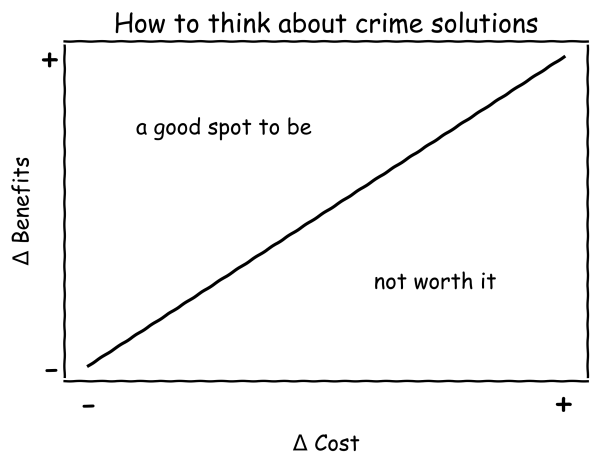
So here we just want Benefits > Costs to justify any particular social program. We can draw this inequality as a diagram, with costs and benefits as the two axes (I will get to the delta triangle symbols in a minute). Any situation in which the benefits are greater than the costs, we are on the good side of the inequality – the top side of the line in the diagram. Social programs that are more costly will need more evidence of benefits to justify investment.

Often we are not examining a program in a vacuum, but are comparing this program to another counter-factual, what happens if that new proposed program does not exist?

Utility_a = Benefits_a - Costs_a : Program A's utility
Utility_s = Benefits_s - Costs_s : Status Quo utility

So here we want in the end for Utility_a > Utility_s – we rather replace the current status quo with whatever this program is, as it improves overall utility. It could be the case that the current status quo is do nothing, which in the end is Utility_s = Benefits_s - Costs_s = 0 - 0 = 0.

It could also be the case that even if Benefits_a > Costs_a, that Utility_a < Utility_s – so in that scenario the program is beneficial, but is worse in overall utility to the current status quo. So in that case even if rated Effective in current CrimeSolutions parlance, a city would not necessarily be better off ponying up the cash for that program. We could also have the situation Benefits_a < Costs_a but Utility_a > Utility_s – that is the benefits of the program are still net negative, but they still have better utility than the current status quo.

So to get whether the new proposed program has added utility over the status quo, we take the difference in two equations:

  Utility_a = Benefits_a - Costs_a : Program A's utility
- Utility_s = Benefits_s - Costs_s : Status Quo utility
--------------------------------------------------------
Δ Utility = Δ Benefits - Δ Costs

And we end up with our changes in the graph I showed before. Note that this implies a particular program can actually have negative effects on crime control benefits, but if it reduces costs enough it may be worth it. For example Megan Stevenson argues pre-trial detention is not worth the costs – although it no doubt will increase crime some, it may not be worth it. Although Stevenson focuses on harms to individuals, she may even be right just in terms of straight up costs of incarceration.

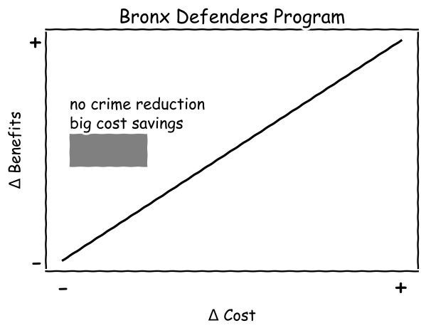
For the Bronx defenders analysis, they showed no benefits in terms of reduced crime. But the intervention was a dramatic cost savings compared to the current status quo. I represent the Bronx defenders results as a grey box in the diagram. It is centered on the null effects for crime benefits, but is clearly in the positive utility part of the graph. If it happened that it was expensive or no difference in costs though, the box would shift right and not clearly be in the effective portion.

For another example, I show the box as not a point in this graph, but an area. An intervention can show some evidence of efficacy, but not reach the p-value < 0.05 threshold. The Chicago summer jobs program is an example of this. It is rated as no effects. I think DSG could reasonably up the sample size requirement for individual recidivism studies, but even if this was changed to the promising or inconclusive recommendation in CrimeSolutions parlance the problem still remains by having a binary yes/no end decision.

So here the box has some uncertainty associated with it in terms of the benefits, but has more area on the positive side of the utility line. (These are just generic diagrams, not meant to be an exact representation, it could be more area of the square should be above the positive utility line given the estimates.) If the authors want to argue that the correct counter-factual status quo is more expensive – so it would shift the pink box to the left – it could as is be a good idea to invest in more. Otherwise it makes sense for the federal govt to invest in more research programs trying to replicate, although from a local govt perspective may not be worth the risk to invest in something like this given the uncertainty. (Just based on the Chicago experiment it probably would be worth the risk for a local govt IMO, but I believe overall jobs and crime programs have a less than stellar track record.)

So these diagrams are nice, but it leaves implicit how CrimeSolutions would in practice measure costs to put this on the diagram. Worst case scenario costs are totally unknown (so would span the entire X axis here, but in many scenarios I imagine people can give reasonable estimates of the costs of social programs. So I believe a simple solution to the current CrimeSolutions issue is two-fold.

  1. They should incorporate costs somewhere into their measurement instrument. This could either be as another weighted term in the Outcome Evidence/Primary Outcomes portion of the instrument, or as another totally separate section.
  2. It should have breakdowns on the website that are not just a single final decision endpoint, but show a range of potential results in a diagram like I show here. So while not quite as simple as the binary yes/no in the end, I believe that policy makers can handle that minor bit of added level of complexity.

Neither of these will make CrimeSolutions foolproof – but better to give suggestions to improve it than to suggest to get rid of it completely. I can forsee issues of defining in this framework what are the relevant costs. So the Stevenson article I linked to earlier talks about individual harm, it may be someone can argue that is not the right cost to calculate (and could do something like a willingness to pay experiment). But that goes for the endpoint outcomes as well – we could argue whether or not they are reasonable for the situation as well. So I imagine the CrimeSolutions/DSG folks can amend the instrument to take these cost aspects into account.

The value of a PhD

For my current work as a data scientist, I spend most of my time writing SQL queries, generating some sort of predictive model on that data using python, and automating those data pipelines using additional command line scripts. Pretty much nothing coding wise I do on a day to day basis I learned in my entire educational career.

The only specific coding classes I took in school were SAS in undergrad and SPSS in grad. All other coding was in Stata and a very tiny bit in R, both incidental to statistical classes. Even those should hardly count, as all it entails is load a dataset and run reg y x or something similar.

That focuses on the software engineering side – the other side of being a data scientist is essentially being an applied mathematician. That may sound fancy, but the work I do I like to think is more akin to accounting with probabilities (where I have to personally create models to estimate the probabilities). While I had extensive quantitative training in graduate school, again nothing I was taught even remotely resembles the mathematics I use on a regular basis at my job.

My social science education entirely focused on causal inference, estimating parameters on the right hand side of the regression equation. I did not cover prediction/forecasting/machine-learning one iota in my classes. I did not even have any classes on cost-benefit analysis, which is more akin to me calculating potential return on investment when I am creating new machine learning models for my company.

The only thing I do regularly at my job you could reasonably point to specific educational training/prep on was presenting results in PowerPoint presentations.

That being said, no way I would be in my current position if I did not have a PhD. For a potential counter-factual, I debated on dropping out of undergrad at one point and going to community college to install HVAC systems. I feel pretty comfortable assuming I would not have ended up as a data scientist if I took that career path. (Before you think to poo-poo on that career path choice, it is easily possible my personal net worth would be in the same ballpark at this point in my life in that counter-factual installing HVAC world. There are significant opportunity costs you are eating when you pursue a PhD.)

So what exactly was the value of my PhD? While you take some classes as a PhD student, I don’t see the main benefit of those as being vocational in nature. When pursuing a PhD it is a full time endeavor, and it is the entire environment that marks it as a major difference from undergraduate education. Pretty much every conversation you have as a PhD student is focused on science.

A second major difference is that you are not a passive consumer of scientific research – you have bridged to becoming a producer of that knowledge. A PhD dissertation by its nature is very sink or swim – you are expected to come up with a particular research topic/agenda, and conduct the appropriate analysis to investigate that particular topic, then share your results with the world. This is very different than working in a job where someone tells you what to do – you show up in the morning and you have 100% latitude to pursue whatever you want.

These two things together I believe are where the value lies in a PhD. The independence necessary to be a successful in a PhD is by its nature not something you can get via prior work experience (unless you count say starting your own business). This coupled with the scientific environment provides an atmosphere where constant learning is necessary to get to the finish line of the dissertation. Even if I still was an academic, it is always necessary for me to consume new material, teach myself new things, and apply that to the work I am pursuing.

So while I did not learn python programming or machine learning in grad school, I just go out, try to consume as much as I can on the material, and apply that knowledge to solve the current problems I am dealing with. There will always be something new I need to teach myself while I am still working, but that is OK. I have the means to teach myself those things from my PhD experience. I am not sure I would have really ever gotten to that point just by focusing on vocational aspects (e.g. taking classes on machine learning or programming) – I think I only got to that point by having to pursue my own independent research.


I’ve been musing this more as potential students ask me whether it is worth it to pursue a PhD. I have mixed feelings, but have settled on this simple dichotomy – if you are only pursuing a PhD because you want to teach, I have grave reservations against recommending a PhD. The supply for these professor positions greatly outpace the demand from universities. So even if you do well as a student, there is no guarantee you will get a tenure track position. In the current market where there are dozens of really good candidates for any position, network effects can dominate that decision.

But, if you are more open to other potential positions, such as public sector researcher positions, think tanks, or private sector data science, I feel more comfortable in saying going for the PhD is a reasonable career choice.

Unfortunately, current education in terms of preparing you to be competitive for private sector data science is somewhat lacking across the social sciences. As I stated at the beginning of this post, I did not personally learn any of the tools I use regularly at my job via traditional education, but more as ancillary to my particular research interests. To follow in my path, the research you pursue needs to somewhat match the skills the current market wants, and these include:

  • predictive modeling (e.g. tree based models, boosted models, deep learning)
  • legitimate coding skills in python/R, as well as tools like git/Docker
  • working with moderately large datasets (SQL, Hadoop, or online AWS)
  • data visualization to explain results/models

I am hoping my former colleagues in social sciences will do a better job of expanding the graduate curricula to better teach these skills. They have utility for the more traditional research as well. I am not holding my breath though for that. So in the meantime if you are pursuing a PhD in the social sciences, and you want to pursue a data science job (or simply hedge in case you cannot land a tenure track gig), these are skills you need to develop on your own while also doing your PhD.

Comparing the WDD vs the Wilson log IRR estimator

So this is maybe my final post on the WDD estimator for the time being (Wheeler & Ratcliffe, 2018). Recently David Wilson had an article in JQC that proposes a different estimator using the same basic information, just pre-post crime counts for treated and control areas (Wilson, 2021). So say we had the table:

         Pre   Post
Treated   50     30
Control   60     55

So in this scenario, my WDD estimate is -20 in the treated area, and -5 in the control area, so the overall estimate is -20 – -5 = -15.

30 - 50 - (55 - 60) = -15

So an estimated reduction of -15 crimes overall. David’s estimator is the logged incident rate ratio (IRR), and so is just like above, except logs all of the values:

log(30) - log(50) - ( log(55) - log(60) ) = -0.4238142

This is a logged incident rate adjustment, so most of the time people exponentiate this value, which is exp(-0.4238142) = 0.6545455. So this suggests crime is reduced by approximately 35% in the treated area relative to the control area in this hypothetical. Or another way to write it is (30/50)/(55/60) = 0.6545455.

So instead of a linear estimate of the total numbers of crimes reduced, this is an estimate of the overall rate reduction. So this begs the question when would you prefer my WDD vs the IRR? I will try to answer that below – in short I think David’s estimator makes sense for meta-analyses (as I have said before in reference to the work in Braga & Weisburd, 2020). But for an individual agency doing an experimental evaluation I much prefer my estimator. The skinny of this logic is that we only really care about the overall crime reduction estimate from a cost-benefit analysis perspective. Backing out this total crime reduction count estimate from David’s IRR estimate can result in some funny business for an individual study.

Identifying Assumptions

So there are really two different assumptions my WDD estimator and David’s IRR estimator make. To generate a standard error estimate around the point estimate for either estimator, both require the data are Poisson distributed. So that makes no difference between the two. The assumption that really distinguishes between the WDD and the IRR estimate is the parallel trends assumption. The WDD assumes parallel trends are on the linear scale, whereas the IRR assumes parallel trends are on the ratio scale.

What exactly does this mean? Imagine we have a treated and control area, but look at the crime trends per time period before the treatment occurred. This set of areas has a set of parallel trends on the linear scale:

Time Treated Control
 0     50      60
 1     40      50
 2     45      55
 3     50      60

When the treated area goes down by 10 crimes, the control area goes down by 10 crimes. That is a parallel on the linear scale. Whereas this scenario is parallel on the ratio scale:

Time Treated Control
 0     50      60
 1     40      48
 2     45      54
 3     50      60

When crime goes down by 20% in the treated area, it goes down by 20% in the control area.

So while this gives a potential way to say you should use the WDD (parallel on the linear scale), or the IRR (parallel on the ratio scale), in practice it is not so simple. For one thing, if you only has the pre/post counts of crime, you cannot distinguish between these two scenarios. You can only tell in the case you have historical data to examine.

For a second part of this, you typically can choose your own control area (see for example the synthetic control estimator). So in most scenarios you could choose a control area to obey the linear or the ratio parallel trends assumption if you wanted to. However it may be in many scenarios there is a natural/easy control area, and you may see what is a better fit in that case for linear/ratio.

A final wee bit of a perverse aspect about this I will mention – pretend we have a treated/control area have approximately the same baseline crime counts/rates:

Time Treated Control
 0      30     30
 1      25     25
 2      20     20
 3      25     25

You actually cannot tell in this scenario whether the parallel trends are on the linear scale for my WDD or the ratio scale for the IRR estimate. They are consistent with either! In practice I think in many cases it will be like this – with noisy data, if you choose a control area that has approximately the same baseline crime counts, it will be quite hard to tell whether the linear parallel trends makes more sense or the ratio parallel trends makes more sense.

There are situations where the linear changes do not make sense, but they tend to be scenarios such as the control area has very little crime (so cannot go below 0 to match larger ups/downs in the treated area). So in that case sure the IRR is plausible and the WDD is not, but those are cases where the control area itself is quite questionable. Also note the IRR is not defined for any cells with 0 crimes – but again it is not good for either of our estimators in that case (although mine won’t fail to spit out a number, the power is so low the number it spits out won’t be worth much).

Bias/Coverage

So I have adapted the same simulation code I used in prior studies/blog posts to evaluate the null distribution and the coverage of David’s IRR estimator. I partly did not pursue it initially back when me and Jerry were discussing this idea, because I thought it would be biased. Generalized linear models are based on maximum likelihood estimators, which are only asymptotically valid. In short it appears I was wrong here and David’s IRR estimator is fine even with just four observations, at least for the handful of scenarios I have tried it (have not looked at very tiny counts of crime, it is undefined if any cell has 0 crimes, as you cannot take the log of 0).

Python code pasted at the very end of the blog post, but for example if we generate a set of null no changes pre/post with a baseline of 50 crimes, the logged irr estimate (converted into a z-score here) is just fine and dandy and has a very close to standard normal distribution based on 10k simulations.

So lets look at the scenario where the control area doesn’t change, but the treated area goes from 50 to 30. We can see again the point estimate in this scenario is spot on the money.

And then we can see the coverage of the logged irr estimator is spot on as well:

So if you are interested in slightly different baseline scenarios, you can use that same simulation code to check out the behavior of David’s estimator and conduct simulated power analysis the same way I have shown for the WDD estimator in prior blog posts.

So if both are unbiased and have good coverage again, why would you prefer the WDD estimator over the IRR estimator (or vice-versa)? Well, lets take the 35% reduction I talked about at the beginning of the post, and the department needs to spend $250k on extra officers to conduct whatever hot spot policing intervention. A 35% reduction may be worth it if we start with a baseline of 200 crimes (so would expect to go down to 130, for a reduction of 70 crimes). If the baseline is 20 crimes, it goes down to 13 crimes (so only a reduction of 7 crimes). The actual benefit of the IRR estimate is entirely dependent on the baseline count of crimes it is applied to.

Even if the IRR estimate is itself unbiased and has proper coverage, for even an individual study backing out the estimated reduction in total crimes from the IRR is biased. So here in this same simulated data (50 to 30 in treated, and 50 to 50 in control areas). The true count reduction is -20, and here is the point estimate on the X axis and the length of the confidence interval for each simulation on the Y axis for my WDD test. You can see they are nicely centered on -20, and the length of the confidence intervals has a very tiny variance – they are mostly just a smidge over 50 in total length. So that is probably tough to wrap your head around, but the variance of the variance estimates for the WDD are small.

Now lets do the same graph for the IRR estimate, but translated back out to a count crime reduction based on the simulated values:

We either have a ton of bias in this estimate (if the estimate of the count reduction is too large, the confidence interval is too small). Or the opposite, the estimate of the count reduction is too small, and the confidence interval is crazy wide. In Andrew Gelman’s terminology, it can result in pretty large type M (magnitude) errors in this simulated example (Gelman & Carlin, 2014). So the variance of the variance estimates in this scenario are quite large.

To be clear – if you are interested in estimating a percent reduction, by all means use David’s IRR estimator. If you however want to translate that percent reduction into an estimate of the total crimes reduced though you should use my WDD estimator in that case. You should not back out a total crimes reduced estimate from the IRR.

Final Thoughts

So I have said a few times I think the IRR estimator makes more sense for meta-analyses. Why do I think that? Well, imagine we have an underlying causal process through which a hot spots policing experiment can randomly deter/prevent a particular proportion of crimes. That underlying causal process suggests an IRR effect. And also the problem I mention with translating back to crime counts I believe should get smaller with tighter estimates.

For a causal process that is more akin to my WDD estimator, imagine some crimes will always be deterred/prevented from a hot spots policing experiment, and some will never be. And we don’t know up-front which is which, so the observed reduction is based on whatever mixture of the two we have at that particular location.

The proportion reduction seems to make more sense to me for active patrol type interventions (which are ephemeral) vs permanent CPTED like interventions which should prevent certain criminal acts in perpetuity. But of course any situation in the real world could have both occurring at the same time.

When you go and look at the meta-analysis of hot spots policing, those interventions are all over the place (Hinkle et al., 2020). I think my WDD estimate would not make sense to mash up into a final meta-analytic estimate. The IRR may not make sense either in the end, but it is plausibly more relevant to compare the IRRs from a study with a baseline of 200 crimes vs one with 40 crimes at baseline. I am not sure it makes sense to compare WDDs in that scenario. But that being said, a few of my blog posts have discussed the WDD normalized per unit area or per unit time. Those normalized estimates are probably more apples to apples in the 200 vs 40 scenario.

A final note I have not discussed here is that David discusses a correction for overdispersion, so that is a potential feather in the cap for his estimator vs the WDD. I’d be a bit hesitant though with that – only four observations to estimate the dispersion term is slicing it a bit thin IMO. But I was wrong about the original estimator, so I may be wrong about that as well. It will take simulation evidence to determine that though – David’s paper just provides the correction term, he doesn’t provide evidence for its utility with small sample data.

And to be fair I have not done simulations to see how my estimator behaves in the presence of overdispersion either. I believe it will simply just cause the standard errors to be too small, so like in Wheeler (2016), I imagine it will just require upping the interval (e.g. use a z-score of 3 instead of 2) to get proper coverage for real crime data.

References

Other Posts of Interest

Python simulation code

Here is a copy-pasted chunk of the entire python simulation code.

'''
Comparing WDD to log(IRR) from Wilson's
recent paper, https://link.springer.com/article/10.1007/s10940-021-09494-w

Andy Wheeler
'''

import pandas as pd
import numpy as np
from scipy.stats import norm
from scipy.stats import poisson
from scipy.stats import uniform
import matplotlib
import matplotlib.pyplot as plt
import os
my_dir = r'D:\Dropbox\Dropbox\Documents\BLOG\wdd_vs_irr'
os.chdir(my_dir)

#########################################################
#Settings for matplotlib

andy_theme = {'axes.grid': True,
              'grid.linestyle': '--',
              'legend.framealpha': 1,
              'legend.facecolor': 'white',
              'legend.shadow': True,
              'legend.fontsize': 14,
              'legend.title_fontsize': 16,
              'xtick.labelsize': 14,
              'ytick.labelsize': 14,
              'axes.labelsize': 16,
              'axes.titlesize': 20,
              'figure.dpi': 100}

matplotlib.rcParams.update(andy_theme)
#########################################################


#This works for the scipy functions as well
np.random.seed(seed=10)

# A function to generate the WDD estimate for simulated data
def wdd_sim(treat0,treat1,cont0,cont1,pre,post):
    tr_cr_0 = poisson.rvs(mu = treat0, size=int(pre)).sum()
    co_cr_0 = poisson.rvs(mu = cont0, size=int(pre)).sum()
    tr_cr_1 = poisson.rvs(mu = treat1, size=int(post)).sum()
    co_cr_1 = poisson.rvs(mu = cont1, size=int(post)).sum()
    # WDD estimates
    est = ( tr_cr_1/post - tr_cr_0/pre ) - ( co_cr_1/post - co_cr_0/pre )
    post2 = (1/post)**2
    pre2 = (1/pre)**2
    var_est = tr_cr_0*pre2 + tr_cr_1*post2 + co_cr_0*pre2 + co_cr_1*post2
    true_val = ( treat1 - treat0 ) - ( cont1 - cont0 )
    z_score = est / np.sqrt(var_est)
    # Wilson log IRR estimates
    true_logirr = np.log( (treat1*cont0) / (cont1*treat0) )
    est_logirr = np.log( ((tr_cr_1/post)*(co_cr_0/pre)) / ( (co_cr_1/post)*(tr_cr_0/pre) ) )
    se_logirr = np.sqrt( 1/tr_cr_1 + 1/co_cr_0 + 1/co_cr_1 + 1/tr_cr_0 )
    z_logirr = est_logirr / se_logirr
    return (tr_cr_0, co_cr_0, tr_cr_1, co_cr_0, est, var_est, true_val, z_score, true_logirr, est_logirr, se_logirr, z_logirr)

def make_data(n, treat0, treat1, cont0, cont1, pre, post):
    base = pd.DataFrame( range(n), columns=['index'])
    base['treat0'] = treat0
    if treat1 is not None:
        base['treat1'] = treat1
    else:
        base['treat1'] = base['treat0']
    if cont0 is not None:
        base['cont0'] = cont0
    else:
        base['cont0'] = base['treat0']
    if cont1 is not None:
        base['cont1'] = cont1
    else:
        base['cont1'] = base['cont0']
    base.drop(columns='index',inplace=True)
    base['pre'] = pre
    base['post'] = post
    sim_vals = base.apply(lambda x: wdd_sim(**x), axis=1, result_type='expand')
    sim_vals.columns = ['sim_t0','sim_c0','sim_t1','sim_c1','est','var_est','true_val','z_score',
                        'true_logirr','est_logirr','se_logirr','z_logirr']
    return pd.concat([base,sim_vals], axis=1)

# Coverage of the log irr estimate
# Lets look at the coverage rate for a decline from 40 to 20
def cover_logirr(data, ci=0.95):
    mult = (1 - ci)/2
    nv = norm.ppf(1 - mult)
    dif = nv*data['se_logirr']
    low = data['est_logirr'] - dif
    high = data['est_logirr'] + dif
    cover = ( data['true_logirr'] > low) & ( data['true_logirr'] < high )
    return cover

# Length of ci for WDD
def len_ci(data, ci=0.95):
    mult = (1 - ci)/2
    nv = norm.ppf(1 - mult)
    dif = nv*np.sqrt( data['var_est'] )
    low = data['est'] - dif
    high = data['est'] + dif
    return low, high, high - low

# Length of ci for IRR estimate on count scale
# This depends on the baseline estimate to multiply
# The IRR by, using the baseline average of the 
# Treatment area

def len_irr(data, ci=0.95):
    mult = (1 - ci)/2
    nv = norm.ppf(1 - mult)
    dif = nv*data['se_logirr']
    low = data['est_logirr'] - dif
    high = data['est_logirr'] + dif
    baseline = data['sim_t0']/data['pre']
    # Even if you use hypothetical, the variance is quite high
    #baseline = data['treat0']
    est_count = baseline*np.exp(data['est_logirr']) - baseline
    c1 = baseline*np.exp(low) - baseline
    c2 = baseline*np.exp(high) - baseline
    return est_count, c1, c2, np.abs(c2 - c1)

##########################
# Example with no change, lets look at the null distribution
sim_n = 10000
no_diff = make_data(sim_n, 50, 50, 50, 50, 1, 1)
no_diff['z_logirr'].describe()
##########################

##########################
# Example with equal time periods, a reduction from 50 to 30 and 50 to 50 in control area
sim_dat = make_data(sim_n, 50, 30, 50, 50, 1, 1)
sim_dat[['true_logirr','est_logirr','se_logirr']].describe()

cl = cover_logirr(sim_dat)
cl.mean()

# Compare length of CI for IRR vs WDD

# WDD length
lowdd, highwdd, lwdd = len_ci(sim_dat)
lwdd.describe()

# IRR length on the count scale
est_cnt_irr, lo_irr, hi_irr, ln_irr = len_irr(sim_dat)
ln_irr.describe()

# Scatterplot of estimated count reduction vs
# Length of CI
fig, ax = plt.subplots(figsize=(8,6))
ax.scatter(est_cnt_irr, ln_irr, c='k', 
            alpha=0.1, s=4)
ax.set_axisbelow(True)
ax.set_xlabel('Estimated Count Reduction [IRR]')
ax.set_ylabel('Length of CI on count scale [IRR]')
plt.savefig('IRR_Len_Est.png', dpi=500, bbox_inches='tight')
plt.show()

# Lets compare to the WDD estimate
fig, ax = plt.subplots(figsize=(8,6))
ax.scatter(sim_dat['est'], lwdd, c='k', 
            alpha=0.1, s=4)
ax.set_axisbelow(True)
ax.set_xlabel('Estimated Count Reduction [WDD]')
ax.set_ylabel('Length of CI on count scale [WDD]')
plt.savefig('WDD_Len_Est.png', dpi=500, bbox_inches='tight')
plt.show()
##########################

How arrests reduce near repeats: Breaking the Chain paper published

My paper (with colleagues Jordan Riddell and Cory Haberman), Breaking the chain: How arrests reduce the probability of near repeat crimes, has been published in Criminal Justice Review. If you cannot access the peer reviewed version, always feel free to email and I can send an offprint PDF copy. (For those not familiar, it is totally OK/legal for me to do this!) Or if you don’t want to go to that trouble, I have a pre-print version posted here.

The main idea behind the paper is that crimes often have near-repeat patterns. That is, if you have a car break in on 100 1st St on Monday, the probability you have another car break in at 200 1st St later in the week is higher than typical. This is most often caused by the same person going and committing multiple offenses in a short time period. So a way to prevent that would on its face be to arrest the individual for the initial crime.

I estimate models showing the reduction in the probability of a near repeat crime if an arrest occurs, based on publicly available Dallas PD data (paper has links to replication code). Because near repeat in space & time is a fuzzy concept, I estimate models showing reductions in near repeats for several different space-time thresholds.

So here the model is Prob[Future Crime = I(time < t & distance < d)] ~ f[Beta*Arrest + sum(B_x*Control_x)] where the f function is a logistic function, and I plot the Beta estimates given different time and space look aheads. Points indicate statistical significance, so you can see they tend to be negative for many different crime and different specifications (with a linear coefficient of around -0.3).

Part of the reason I pursued this is that the majority of criminal justice responses to near repeat patterns in the past were target hardening or traditional police patrol. Target hardening (e.g. when a break in occurs, go to the neighbors and tell them to lock their doors) does not appear to be effective, but traditional patrol does (see the work of Rachel/Robert Santos for example).

It seems to me ways to increase arrest rates for crimes is a natural strategy that is worthwhile to explore for police departments. Easier said than done, but one way may be to prospectively identify incidents that are likely to spawn near repeats and give them higher priority in assigning detectives. In many urban departments, lower level property crimes are never assigned a detective at all.

Open Data and Reproducible Criminology Research

This is part of a special issue put together by Jonathan Grubb and Grant Drawve on spatial approaches to community violence. Jon and Grant specifically asked contributors to discuss a bit about open data standards and replication materials. I repost my thoughts on that here in full:

In reference to reproducibility of the results, we have provided replication materials. This includes the original data sources collated from open sources, as well as python, Stata, and SPSS scripts used to conduct the near-repeat analysis, prepare the data, generate regression models, and graph the results. The Dallas Police Department has provided one of the most comprehensive open sources of crime data among police agencies in the world (Ackerman & Rossmo, 2015; Wheeler et al., 2017), allowing us the ability to conduct this analysis. But it also identifies one particular weakness in the data as well – the inability to match the time stamp of the occurrence of an arrest to when the crime occurred. It is likely the case that open data sources provided by police departments will always need to undergo periodic revision to incorporate more information to better the analytic potential of the data.

For example, much analysis of the arrest and crime relationship relies on either aggregate UCR data (Chamlin et al., 1992), or micro level NIBRS data sources (Roberts, 2007). But both of these data sources lack specific micro level geographic identifiers (such as census tract or addresses of the events), which precludes replicating the near repeat analysis we conduct. If however NIBRS were to incorporate address level information, it would be possible to conduct a wide spread analysis of the micro level deterrence effects of arrests on near repeat crimes across many police jurisdictions. That would allow much broader generalizability of the results, and not be dependent on idiosyncratic open data sources or special relationships between academics and police departments. Although academic & police practitioner relationships are no doubt a good thing (for both police and academics), limiting the ability to conduct analysis of key policing processes to the privileged few is not.

That being said, currently both for academics and police departments there are little to no incentives to provide open data and reproducible code. Police departments have some slight incentives, such as assistance from governmental bodies (or negative conditions for funding conditional on reporting). As academics we have zero incentives to share our code for this manuscript. We do so simply because that is a necessary step to ensure the integrity of scientific research. Relying on the good will of researchers to share replication materials has the same obvious disadvantage that allowing police departments to pick and choose what data to disseminate does – it can be capricious. What a better system to incentivize openness may look like we are not sure, but both academics and police no doubt need to make strides in this area to be more professional and rigorous.

Podcast and Video Shout Outs

So y’all know I really enjoy blogs. So much so I think they often have a higher value added than traditional peer review papers. There are other mediums I would like to recognize, and those are Podcasts and video tutorials. So while I like to do lab tutorials (pretty much like my blog posts in which I step through some code), I know many students would prefer I do videos and lectures. And I admit some of these I have seen done quite well on Coursera for example.

Another source I have been consuming quite a bit lately are Podcasts. These often take the form of an interview. So are not technical in nature, but are more soft story telling, such as talking about a particular topical area the interviewee is expert in, or that persons career path. So here are my list of these resources I have personally learned from and enjoyed.

None of these I have listened/watched 100% of the offerings, but have listened/watch multiple episodes (and will continue to listen/watch more)! These are very criminal justice focused, so would love to branch out to data science and health care resources if folks have suggestions!

Podcasts

Reducing Crime – Jerry Ratcliffe interviews a mix of academics and folks working in the criminal justice field. I have quite a few of these episodes I found personally very informative. John Eck, Kim Rossmo, and Phil Goff were perhaps my favorites of academics. Danny Murphy and Thomas Abt were really good as well (for my favorite non-academics offhand).

Niro Knowledge – Nicholas Roy is a current crime analyst, and interviews other crime analysts and academics. Favorite interviews so far are Cynthia Lum and Renee Mitchell. Similar to reducing crime is typically more focused on a particular topic of interest to the person being interviewed (e.g. Renee talked about her work on crime harm indices).

Analyst Talk – This is a podcast hosted by Jason Elder where he interviews crime analysts from all over about their careers. Annie Thompson and my former colleague Shelagh Dorn’s are my favorite so far, but I also need to listen in sometime on Sean Bair’s series of talks as well.

Abt Podcasts – This I only came across a week ago, but have listened to several on data science, CJ, and social determinants of health. These are a bit different than the other podcasts here, they are shorter and have two individuals from different fields discuss social science relevant to the chosen topic.

Videos

Canadian Society of Evidence Based Policing – Has many interviews of academics in crim/cj. I have an interview with them (would not recommend, I need to work on sitting still!) I really enjoyed the Peter Neyroud interview though is my favorite.

UARK CASDAL – These are instructional videos uploaded by Grant Drawve, mostly around doing crime analysis in Excel, but also has a few in ArcGIS.

StatQuest with Josh Starmer – This is one of the few non crim/cj examples I watch regularly. As interview questions at my work place for entry data scientists we often ask folks to explain machine learning models (such as random forests or XGBoost) in some simple terms. These videos are excellent resources to get you to understand the basics of the mathematics behind the techniques.

Again let me know if of podcasts/video series I am missing out on in the comments!

Reproducible research and code review for journals

Recently came across two different groups broaching the subject of code reviews and reproducible research more broadly for criminal justice. There are certainly aspects of either that make it difficult in the context of peer review. But I am not one to let the perfect be the enemy of the good, so I will layout the difficulties and give some comments on potential good enough solutions that still make marked improvements on the current state of affairs in crim/cj research.

Reproducible Research

So what do I mean by reproducible research? Jeromy Anglim on crossvalidated has a good breakdown on different ways we may apply the term. So to some it may mean if you did a hot spots policing experiment, can I replicate the same crime reduction results in another city.

These are important to publish (simply because social science experiments will inevitably have quite a bit of variance), but this is often not what we are talking about when we talk about replication. We are often talking about a much smaller in scope goal – if I give you the exact same data, can you reproduce the tables/figures in the manuscript you used to make your inferences?

One problem that is often the case with CJ research is that we are working with sensitive data. If I do analysis on a survey of a sensitive topic, I often cannot share the data. But, I do not believe that should entirely put a spike in the question of reproducible data. I have broken down different levels that are possible in making research more reproducible:

  1. A Sharing data and code files to reproduce the paper results
  2. B Sharing code files and simulated data that illustrate the results
  3. C Sharing the plain-text log files showing the code and results of tables/figures

So I have not seen C proposed anywhere, but it is a dead simple solution that almost everyone should be able to accommodate. It simply involves typing log using "output.txt", text at the top of your Stata file, or OUTPUT EXPORT /PDF DOCUMENTFILE="output.pdf" at the end of your SPSS analysis (or could be done via the GUI), etc. These are the log/output files used to generate the results you report in the paper, and typically contain both the commands run, as well as the resulting tables. These files can quite easily not contain privileged information (in fact they won’t be default most of the time, unless you printed out individual names in a table for example in intermediate results).

To accomplish C does take some modicum of wherewithal in terms of writing code, but it is a pretty low bar. So I see no reason why all quantitative analyses cannot require at least this step right now. I realize it is not foolproof – a bad actor could go and edit the results (same as they could edit the results without this information). But it ups the level of effort to manipulate results by quite a bit, and more importantly has the potential to catch more mundane transcription errors that occur quite frequently.

Sometimes I want more details on the code used, the nature of the data etc. (Most quasi-experimental design for example can be summed up as shape your data in a special way and run a particular regression model.) For people like me who care about that, B helps with that, in that I can see the code front-to-back, can actually go and inspect the shape and values in a particular rectangular dataset, and see how the code interacts with those objects. The only full on example of this I am aware of is a recent example paper in Nature Behavior that shares the code using simulated data.

B is also very similar to people who release statistical packages to reproduce their code. So if you release an R package that conducts your new fancy technique, even if you can’t share your data it is really good for people to be able to view the underlying code even by itself to understand the technique better and in conjunction build on your work more. If you do a new technique, it is a crazy ton of work to replicate that on your own, so most people will not bother.

A is most of the way there to the gold standard – if you can share both the data and the code used to reproduce the analysis. Both A and B take a significant amount of knowledge of statistical programming to accomplish. Most people in our field do not have the skills to write an analysis front-to-back that can run in a series of scripts though. To get to A/B grad programs in crim/cj need to spend crazy more time on teaching these skills, which is near zero now almost across the board.

One brief thing to mention about A is that the boundary is difficult to define. So for example, I share code to reproduce analysis in my 311 and crime at micro places in DC paper (paper link, code). But this starts from a dataset that has the street units in DC and all of the covariates already compiled. But where did that dataset come from? I created it by compiling many different sources, so the base dataset is itself very difficult to replicate. Again not letting the perfect be the enemy of the good, I think just starting from your compiled dataset, and replicating the tables/graphs in the manuscript is better than letting the fuzzy boundary prevent you from sharing anything.

Code Reviews for Journal Submissions

The hardest part of A is that even after you share your data, some journals want to be able to run the code locally to entirely reproduce your results. So while I have shared data code (A above) for many papers, see this spreadsheet, they have not been externally vetted by any of those journals. This vetting is the standard in some economic journals now I believe, and would not be surprised in some poli-sci journals as well. This is a very hard problem though, and requires significant resources from both the journal and the researcher to be able to do that.

The biggest hurdle is that even if you share your data/code, your particular system may be idiosyncratic. You may have different R libraries installed than me. You may have different versions of python packages. I may have used a program on Windows to do some analysis you cannot do on a Mac. You may rely on some paid API I cannot access.

These are often solvable problems, but take quite a bit of time to work out. A comparable example to my work is when data scientists say ‘going to production’. This often involves taking some analysis I did on my local machine, and making it run autonomously on my companies servers. There are some things that make it more or less difficult than the typical academic situation, but I think it is broadly comparable. To go to production for a project will typically take me 3-6 months at 50% of my time, so maybe something like 300 hours for a lowish end estimate. And that is just the time it takes from the researchers end, from the journals end it will also take a significant amount of time to compile every ones code and verify the results.

Because of this, I don’t think the fully reproducible re-run my code and generate the exact same tables are feasible in the current way we do academic research and peer review. But again that is why I list C above – we shouldn’t let the perfect be the enemy of the good.

Validating New Empirical Techniques

The code review above is not really code review in the sense that someone looks at your code and says this is correct, it is simply just saying can I get the same results as you. You may want peer review to accomplish the task of not only saying is it reproducible, but is it valid/correct? There are a few things towards this end I would like to see more often in crim/cj. I realize we are not statistics, so cannot often ask for formal proofs. But there are simpler things we can do to verify the results. These are the responsibility of the researcher to provide, not the reviewer to script up on their own to validate someone elses work.

One, illustrate the technique using a very simplified example. So for instance, in my p-median patrol areas paper, I show an example of constructing the linear program with only four areas. You should be able to calculate what the result should be by hand, so can verify the correctness of your algorithm. This has the added benefit of being a very good pedagogical way to describe your method.

Two, illustrate the technique on a larger sample of simulated data in which you again know the correct result. For one example of this, I showed how to estimate group based trajectory models using deep learning libraries. Again your model/method should be able to recover the correct result (which you know) given the simulated fake data.

Three, validate the result using real data compared to the current standard. For crime mapping papers, this means comparing forecasts compared to RTM, or simpler regression models, or simply prior crime = future crime on out of sample data. Amazingly many machine learning papers in CJ do not do out of sample predictions. If it is an inferential procedure, comparing the results to some other status quo technique is similar, such as showing conformal prediction intervals have smaller widths (so more statistical power) than placebo results for synthetic control designs (at least for that example with state panel level crime data).

You may not have all three of these examples in any particular paper, but I think for very new techniques 1 or 2 is necessary. 3 is often a by-product on the analysis anyway. So I do not believe any of these asks are that onerous. If you have the skills to create some new technique, you should be able to accomplish 1 or 2.

I do not have any special advice in terms of the reviewers perspective. When I do code reviews at work, what we do is go line by line, and my co-workers give high level design advice. E.g. you should use a config file for this instead of defining it inline, you should turn this block into a function, you should make a class to open/close the database connections etc. The code reviews do not validate the technical correctness, so if I queried the wrong data they wouldn’t know in the code review. The proof is in the pudding so to speak, so if my results are performing really badly in the real world I know I am doing something wrong. (And the obverse, if my results are on the mark and making money I am pretty sure I did nothing terribly wrong.)

Because there are not these real world mechanisms to validate code in peer reviewed papers, my suggestions for 1/2/3 are the closest I think we can get in many circumstances. That and simply making your code available will dramatically improve the reproducibility and validity of your research compared to the current status quo in our field.

My online course lab materials and musings about online teaching

I often refer folks to the courses I have placed online. Just for an update for everyone, if you look at the top of my website, I have pages for each of my courses at the header of my page. Several of these are just descriptions and syllabi, but the few lab based courses I have done over the years I have put my materials entirely online. So those are:

And each of those pages links to a GitHub page where all the lab goodies are stored.

The seminar in research focuses on popular quasi-experimental designs in CJ, and has code in R/Stata/SPSS for the weekly lessons. (Will need to update with python, I may need to write my own python margins library though!)

Grad GIS is mostly old ArcGIS tutorials (I don’t think I will update ArcPro, will see when Eric Piza’s new book comes out and just suggest that probably). Even though the screenshots are perhaps old at this point though the ideas/workflow are not. (It also has some tutorials on other open source tools, such as CrimeStat, Jerry’s Near Repeat Calculator, GeoDa, spatial regression analysis in R, and Mallesons/Andresens SPPT tool are examples I remember offhand.)

Undergrad Crime Analysis is mostly focused on number crunching relevant to crime analysts in Excel, although has a few things in Access (making SQL queries), and making a BOLO in publisher.

So for folks self-learning of course use those resources however you want. My suggestion is to skim through the syllabus, see if you want to learn about any particular lesson, and then jump right to that one. No need to slog through the whole course if you are just interested in one specific thing.

They are also freely available to any instructors who want to adapt those materials for their own courses as well.


One of the things that has disappointed me about the teaching response to Covid is instead of institutions taking the opportunity to really invest in online teaching, people are just running around with their heads cut off and offering poor last minute hybrid courses. (This is both for the kiddos as well as higher education.)

If you have ever taken a Coursera course, they are a real production! And the ones I have tried have all been really well done; nice videos, interactive quizzes with immediate feedback, etc. A professor on their own though cannot accomplish that, we would need investment from the University in filming and in scripting the webpage. But once it is finished, it can be delivered to the masses.

So instead of running courses with a tiny number of students, I think it makes more sense for Universities to actually pony up resources to help professors make professional looking online courses. Not the nonsense with a bad recorded lecture and a discussion board. It is IMO better to give someone a semester sabbatical to develop a really nice online course than make people develop them at the last minute. Once the course is set up, you really only need to administer the course, which takes much less work.

Another interested party may be professional organizations. For example, the American Society of Criminology could make an ad-hoc committee to develop a model curriculum for an intro criminology course. You can see in my course pages I taught this at one point – there is no real reason why every criminology teacher needs to strike out on their own. This is both more work for the individual teacher, as well as introduces quite a bit of variation in the content that crim/cj students receive.

Even if ASC started smaller, say promoting individual lessons, that would be lovely. Part of the difficulty in teaching a broad course like Intro to Criminology is that I am not an expert on all of criminology. So for example if someone made a lesson plan/video for bio-social criminology, I would be more apt to use that. Think instead of a single textbook, leveraging multi-media.


It is a bit ironic, but one of the reasons I was hired at HMS was to internally deliver data science training. So even though I am in the private sector I am still teaching!

Like I said previously, you are on your own for developing teaching content at the University. There is very little oversight. I imagine many professors will cringe at my description, but one of the things I like at HMS is the collaboration in developing materials. So I initially sat down with my supervisor and project manager to develop the overall curricula. Then for individual lessons I submit my slides/lab portion to my supervisor to get feedback, and also do a dry run in front of one of my peers on our data science team to get feedback. Then in the end I do a recorded lecture – we limit to something like 30 people on WebEx so it is not lagging, but ultimately everyone in the org can access the video recording at a later date.

So again I think this is a better approach. It takes more time, and I only do one lecture at a time (so take a month or two to develop one lecture). But I think that in the end this will be a better long term investment than the typical way Uni’s deliver courses.

New book: Micro geographic analysis of Chicago homicides, 1965-2017

In joint work with Chris Herrmann and Dick Block, we now have a book out – Understanding Micro-Place Homicide Patterns in Chicago (1965 – 2017). It is a Springer Brief book, so I recommend anyone who has a journal article that is too long that this is a potential venue for the work. (Really this is like the length of three journal articles.)

A few things occurred to prompt me to look into this. First, Chicago increased a big spike of homicides in 2016 and 2017. Here is a graph breaking them down between domestic related homicides and all other homicides. You can see all of the volatility is related to non-domestic homicides.

So this (at least to me) begs the question of whether those spiked homicides show similar characteristics compared to historical homicides. Here we focus on long term spatial patterns and micro place grid cells in the city, 150 by 150 meter cells. Dick & Carolyn Block had collated data, including the address where the body was discovered, using detective case notes starting in 1965 (ending in 2000). The data from 2000 through 2017 is the public incident report data released by Chicago PD online. Although Dick and Carolyn’s public dataset is likely well known at this point, Dick has more detailed data than is released publicly on ICPSR and a few more years (through 2000). Here is a map showing those homicide patterns aggregated over the entire long time period.

So we really have two different broad exploratory analyses we employed in the work. One was to examine homicide clustering, and the other was to examine temporal patterns in homicides. For clustering, we go through a ton of different metrics common in the field, and I introduce even one more, Theil’s decomposition for within/between neighborhood clustering. This shows Theil’s clustering metric within neighborhoods in Chicago (based on the entire time period).

So areas around the loop showed more clustering in homicides, but here it appears it is somewhat confounded with neighborhood size – smaller neighborhoods appear to have more clustering. This is sort of par for the course for these clustering metrics (we go through several different Gini variants as well), in that they are pretty fickle. You do a different temporal slice of data or treat empty grid cells differently the clustering metrics can change quite a bit.

So I personally prefer to focus on long term temporal patterns. Here I estimated group based trajectory models using zero-inflated Poisson models. And here are the predicted outputs for those grid cells over the city. You can see unlike prior work David Weisburd (Seattle), myself (Albany), or Martin Andresen (Vancouver) has done, they are much more wavy patterns. This may be due to looking over a much longer horizon than any of those prior works though have.

The big wave, Group 9, ends up being clearly tied to former large public housing projects, which their demolitions corresponds to the downturn.

I have an interactive map to explore the other trajectory groups here. Unfortunately the others don’t show as clear of patterns as Group 9, so it is difficult to answer any hard questions about the uptick in 2016/2017, you could find evidence of homicides dispersing vs homicides being in the same places but at a higher intensity if you slice the data different ways.

Unfortunately the analysis is never ending. Chicago homicides have again spiked this year, so maybe we will need to redo some analysis to see if the more current trends still hold. I think I will migrate away from the clustering metrics though (Gini and Theil), they appear to be too volatile to say much of anything over short term patterns. I think there may be other point pattern analysis that are more diagnostic to really understand emerging/changing spatial patterns.

The coffee next to the cover image is Chris Herrmann’s beans, so go get yourself some as well at Fellowship Coffee!